Sequence alignment I
alignment dynamic programming
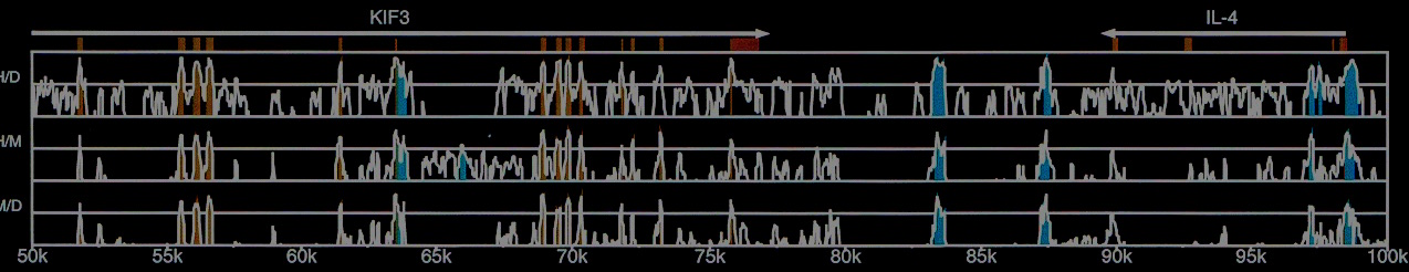
The cover image shows pairwise alignments for human, mouse, and dog KIF3 locus from Dubchak et al. 2000.
WarmUp with Python Loops
- Open this notebook
- Make a copy of it in your drive
- Go through it and execute all cells
Introduction to dynamic programming
(Based on dynamic programming examples from InteractivePython) and excellent alignment lecture materials from Ben Langmead.
Suppose you are a cashier who’s job is, generally speaking, to receive money and to give out change. Suppose that someone buys something that costs \$9.37 and gives you a 10 dollar bill. You need to give \$0.63 back in smallest possible number of coins. The US coin denominations are:
- 100 (1 dollar)
- 50 (half-dollar)
- 25 (quarter)
- 10 (dime)
- 5 (nickel)
- 1 (penny)
So, given these coins you will:
- start with the largest coin smaller than the amount you need to give back = 50 Cents
- repeat for the remaining $0.13 and select 10 Cents (NOTE: this is recursion happening)
- finish with three 1 cent counts thus you ended up with 5 (50 + 10 + 3 × 1) coins.
Solving problem exhaustively
Now (as suggested here) suppose you are a cashier in a strange country where there is also a 21 cent coin in circulation. By using the algorithm above, you will still give your customer five coins, while the “correct” solution will certainly be giving him/her three 21 cent coins. So the algorithm we used above simply does not work.
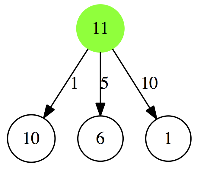
Let’s rephrase the problem. The smallest number of coins summing up to $0.63 cents (in our strange country with a 21 cent coin) will be:
- a minimal collection of coins summing up to $0.62 plus a 1 cent coin
- a minimal collection of coins summing up to $0.58 plus a 5 cent coin
- a minimal collection of coins summing up to $0.53 plus a 10 cent coin
- a minimal collection of coins summing up to $0.42 plus a 21 cent coin
- a minimal collection of coins summing up to $0.38 plus a 25 cent coin
- a minimal collection of coins summing up to $0.13 plus a 50 cent coin
 |
| Figure 1A. 1. First iteration |
Next, for each of these possibilities we will repeat this again. For example for $0.62 will consider:
- a minimal collection of coins summing up to $0.61 plus a 1 cent coin
- a minimal collection of coins summing up to $0.57 plus a 5 cent coin
- a minimal collection of coins summing up to $0.52 plus a 10 cent coin
- a minimal collection of coins summing up to $0.41 plus a 21 cent coin
- a minimal collection of coins summing up to $0.37 plus a 25 cent coin
- a minimal collection of coins summing up to $0.12 plus a 50 cent coin
 |
| Figure 1B. 2. Second iteration |
And again. For $0.58 we will have:
 |
| Figure 1C. 3. Third iteration. Note that amounts highlighted in red are repeated. Below we explain why this is really bad. |
and so on. Basically, as every iteration we are trying to find:
While this algorithm will find us the smallest number of coins necessary to give out a particular amount in change, it does this at a horrific price: it is extremely inefficient as it recomputes all possibilities at every iteration. For instance, if we ask the algorithm to compute the minimal number of coins necessary to give out 63 cents in change in a country with only four coins (1, 5, 10, and 25 cents) it will take 67,716,925 iterations (recursive calls). As a result you will probably loose all of your customers while they are waiting for the change.
The code snippet below implements this algorithm (do not worry if you don’t quire understand python. It is OK for now). If you execute it (press the play button) your browser will likely crash as it will get tired waiting for result to come back (try it anyway):
# Import time function to check the speed of our code
from time import time

# Below we are defining function that takes two arguments:
#   coinValueList - the list of coins circulating in your country of choice
#   change - the amount of change that needs to be given
# It return the smallest number of coins in which this amount of change can
# be given

def recMC(coinValueList,change):
   minCoins = change

   if change in coinValueList:
     return 1
   else:
      for i in [c for c in coinValueList if c <= change]:
         numCoins = 1 + recMC(coinValueList,change-i)
         if numCoins < minCoins:
            minCoins = numCoins
   return minCoins

st = time()
print(recMC([1,3],4))
print('Took %0.3f seconds' % (time() - st))
Caching helps a bit
One potential way to solve our problem in a reasonable amount of time is to take advantage of red nodes shown in Fig. 1C above. What if before calling the function we check if a minimum number of coins for a particular amount was already computed? Apparently this speeds things up quite dramatically:
from time import time

def recDC(coinValueList,change,knownResults):
   minCoins = change
   if change in coinValueList:
      knownResults[change] = 1
      return 1
   elif knownResults[change] > 0:
      return knownResults[change]
   else:
       for i in [c for c in coinValueList if c <= change]:
         numCoins = 1 + recDC(coinValueList, change-i,
                              knownResults)
         if numCoins < minCoins:
            minCoins = numCoins
            knownResults[change] = minCoins
   return minCoins

st = time()
print(recDC([1,5,10,25],63,[0]*64))
print('Took %0.3f seconds' % (time() - st))
Now you can see that it takes under a second to find that it takes 3 coins to give 63 cents in change in a country with 1, 5, 10, 21, and 25 cent coins. Yet this script still makes 221 calls (better than 67,716,925, but still a lot) for find the answer.
Introducing dynamic programming
Let’s flip things around. Instead of starting from 63 cents and going down through the tree as shown in Fig. 1A-C we will instead compute the minimal number of coins for every value from 1 to 63. To save space, let’s instead assume that we need to give 11 cents in change. Let’s compute a dynamic programming array for minimal number of coins between 1 and 11:
| Amount | Minimal Number of Coins |
|---|---|
| 0 | 0 |
| 1 | 1 |
| 2 | 2 |
| 3 | 3 |
| 4 | 4 |
| 5 | 1 |
| 6 | 2 |
| 7 | 3 |
| 8 | 4 |
| 9 | 5 |
| 10 | 1 |
| 11 | 2 |
for amounts between 1 and 4, we have no choice, since we have only pennies. At 5 we can either use 5 pennies or 1 nickel. According to this strategy (for a country with 1, 5, 10, and 25 cent coins):
nickel wins (needs just 1 coin). From 6 to 9 we can either use all pennies (values will be 6, 7, 8, and 9) or a combination of nickel and pennies (values will be 2, 3, 4, 5). Again, smaller values win.
Let’s now use this table to decide what is the minimum number of coins necessary to give 11 cents in change:
 |
| Figure 2. Making change for 11 cents. Let’s look at leftmost branch. If you give 1 cent in change, you are left with 10 more to give. You consult Table 1 above and see that 10 cents can be given with 1 coin, so it will be 1 + 1 = 2 coins. In the center branch we give 5 cents in one coin and have 6 more cents to give. Looking at Table 1 tells us that 6 cents can be given in 2 coins, so 1 + 2 = 3 coins. Finally, in the rightmost branch giving 10 cents as one coin leaves 1 cent to give in change, which is also 1 coin, so 1 + 1 = 2. Thus we can either give 10 cents + 1 cent or 1 cent + 10 cents, which is equivalent since in both cases we give only 2 coins. |
The following python code implements a function called dynamicCoinChange which computes a table (like Table 1) for any amount. In line 20 of the script we print a value corresponding to the amount we need to give back. That value is the minimum number of coins. Note that this program takes virtually no time to run.
from time import time

def dynamicCoinChange( coins, amount ):

	table = [ 0 for i in range( 0, amount+1 ) ]

	n = len( coins )
	for i in range( 1, amount+1 ):
		smallest = float( "inf" )
		for j in range( 0, n ):
			if ( coins[j] <= i ):
				smallest = min(smallest, table[i - coins[j]])
		table[i] = 1 + smallest
	return table

amount = 63
money = [1,5,10,21,25]
da = dynamicCoinChange(money, amount)

print("It takes {} coins to give out {} cents".format(da[amount],amount))

st = time()
print('Took %0.3f seconds' % (time() - st))So, dynamic programming is a methodology where complex problems are broken down to simple subproblems, that are computed just once and then used to solve the complete problem. In this example, we first pre-compute the number of coins needed to make change for any amount up to the required one, and then produce the answer.
Sequence alignment
We have just seen the principle behind dynamic programming. This approach is also extremely useful for comparing biological sequences, which is coincidentally one of the main points of this course. This lecture explain how this is done. In writing this text I heavily relied on wonderful course taught by Ben Langmead at Johns Hopkins.
How different are two sequences?
Suppose you have two sequences of the same length:
A C A T G C C T A
A C T G C C T A C
How different are they? In other words, how many bases should be change to turn one sequence onto the other:
A C A T G C C T A
| | * * * | * * *
A C T G C C T A C
the vertical lines above indicate positions that are identical between the two sequences, while asterisks show differences. It will take six substitutions to turn one sequence into the other. This number – six substitutions – is called Hamming distance or the minimal number of substitutions required to turn one string into another. The code below computes the Hamming distance. Try it. You can change seq1 and seq2 into whatever you want except that they should have the same length.
def hammingDistance(x, y):
    ''' Return Hamming distance between x and y '''
    assert len(x) == len(y)
    nmm = 0
    for i in range(0, len(x)):
        if x[i] != y[i]:
            nmm += 1
    return nmm

# You can change seq1 and seq2 to whatever you want
# But make sure that they are of the same length

seq1 = 'ACATGCCTA'
seq2 = 'ACTGCCTAC'

hamDist =  hammingDistance(seq1, seq2)

print("The Hamming distance between {} and {} is {}".format(seq1, seq2, hamDist))
Now in addition to substitutions (i.e., changing one character into another) let’s allow instertions and deletions. This will essentially allow us to insert dashes (gaps) between characters:
A C A T G C C T A -
| | * | | | | | | *
A C - T G C C T A C
In this case the edit distance between two sequences is 2. It is defined as the minimum number of operations (substitutions, insertions, and deletions) requited to turn one string into another. The compared strings do not have to be of the same length to be able to compute the edit distance as we can compensate for length differences using deletions and insertions. While the situation above (where we inserted two dashes) is biologically much more meaningful (and realistic), it is much more difficult to find.
Generalizing the problem
Before we can develop an algorithm that will help us to compute the edit distance let’s develop a general framework that would allow us to think about the problem in exact terms. Let’s look at a pair of VERY long sequences. So long, that we do not even see the left end – it disappears into $\infty$:
the red parts of the two sequences represent prefixes for the last nucleotides shown in black. Let’s assume that the edit distance between the two prefixes is known (don’t ask how we know, we just do). For simplicity let’s “compact” the prefix of the first sequence into $\alpha$ and the prefix of the second sequence into $\beta$:
again, the edit distance between $\alpha$ and $\beta$ is known to us. The three possibilities for computing the edit distance between $\alpha G$ and $\beta C$ are:
but we not always have $\texttt{G}$ and $\texttt{C}$ as two last nucleotiodes, so for the general case:
where $\delta(x,y) = 0$ if $x = y$ (nucleotides match) and $\delta(x,y) = 1$ if $x \neq y$ (nucleotides do not match). The $\delta(x,y)$ has a particular meaning. If the two nucleotides at the end are equal to each other, there is nothing to be done – no substitution operation is necessary. If a substitution is necessary however, we will record this by adding 1. When we will be talking about global and local alignment below the power of $\delta(x,y)$ will become even more clear.
Recall the change problem from the above. We can write an algorithm that would exhaustively evaluate the above expression for all possible suffixes. This algorithm is below. Try executing it. It will take roughly ~2 seconds to find the edit distance between the two sequences used above:
# Import time function to check the speed of our code
from time import time

def edDistRecursive(x, y):
    global n
    if len(x) == 0: return len(y)
    if len(y) == 0: return len(x)

    delt = 1 if x[-1] != y[-1] else 0
    return min(edDistRecursive(x[:-1], y[:-1]) + delt,
               edDistRecursive(x[:-1], y) + 1,
               edDistRecursive(x, y[:-1]) + 1)
st = time()
print(edDistRecursive("ACATGCCTA","ACTGCCTAC"))
print('Took %0.3f seconds' % (time() - st))
Again, don’t worry if Python looks scary to you. The take-home-message here is that it takes a very long time to compute the edit distance between two sequences that are only nine nucleotides long! Why is this happening? Fig. 3 below shows a small subset of situations the algorithm is evaluating for two very short strings $\texttt{TAG}$ and $\texttt{TAC}$:
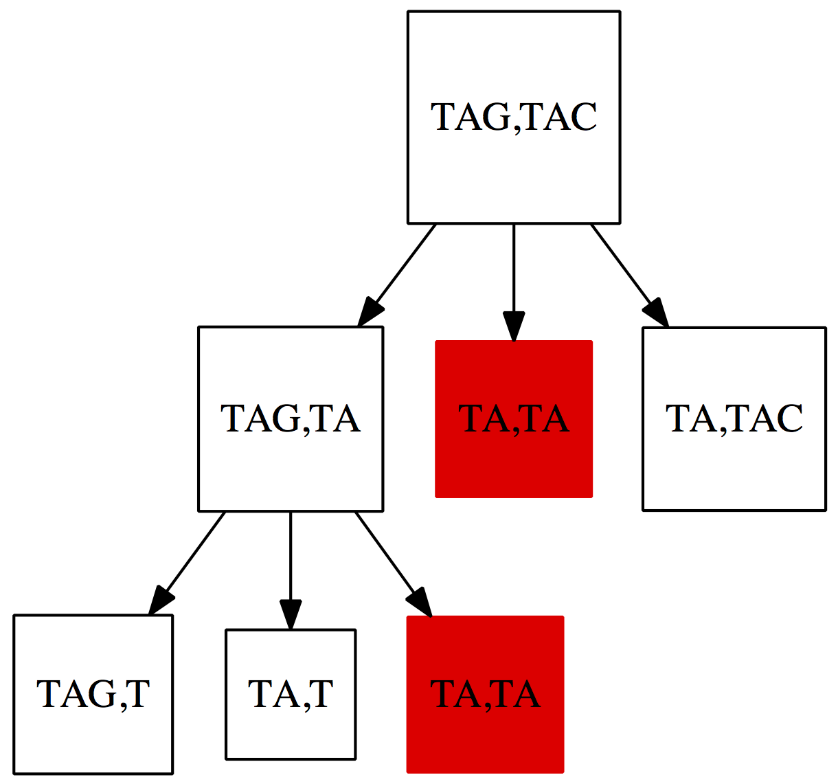 |
| Figure 3. A fraction of situations evaluated by the naïve algorithm for computing the edit distance. Just like in the case of the change problem discussed in the previous lecture a lot of time is wasted on computing distances between suffixes that has been seen more than once (shown in red). |
To understand the magnitude of this problem let’s look at slightly modified version of the previous Python code below. All we do here is keeping track how many times a particular pair of suffixes (in this case $\texttt{AC}$ and $\texttt{AC}$) are seen by the program. The number is staggering: 48,639. So this algorithm is extremely wasteful.
# Import time function to check the speed of our code
from time import time

n = 0

def edDistRecursive(x, y):
    global n
    if len(x) == 0: return len(y)
    if len(y) == 0: return len(x)

    # Let's keep track of how many times prefix TA is seen

    if x == 'TA' and y == 'TA':
      n += 1
    delt = 1 if x[-1] != y[-1] else 0
    return min(edDistRecursive(x[:-1], y[:-1]) + delt,
               edDistRecursive(x[:-1], y) + 1,
               edDistRecursive(x, y[:-1]) + 1)
st = time()
print(edDistRecursive("TAG","TAC"))
print('Took %0.3f seconds' % (time() - st))
print("TA,TA is seen {} times".format(n))
While this approach to the edit distance problem is correct, it will hardly help us on the genome-wide scale. Just like in case of the change problem dynamic programming is going to save the day.
Dynamic programming to the rescue
Our goal is to find an optimal alignment between two sequences. Note that so far this is the first time we use the term alignment in this section. It turns out that in order to find the alignment we first need to learn how to compute edit distances between sequences efficiently. So, suppose we have two sequences that deliberately have different lengths:
$\texttt{G C T A T A C}$
and
$\texttt{G C G T A T G C}$
Let’s represent them as the following matrix where the first character $\epsilon$ represents an empty string:
Let’s fill the first column and first raw of the matrix. Because the distance between a string and an empty string is equal to the length of the string (e.g., a distance between string $\texttt{TCG}$ and an empty string is 3) this resulting matrix will look like this:
Now, let’s fill in the cell between $\texttt{G}$ and $\texttt{G}$. Recall that:
where $\delta(x,y) = 0$ if $x = y$ and $\delta(x,y) = 1$ if $x \neq y$. And now let’s color each of the cells corresponding to each part of the above expression:
In this specific case:
This minimum of 0, 2, and 2 will be 0, so we are putting zero into that cell:
Using this uncomplicated logic we can fill the entire matrix like this:
The lower rightmost cell highlighted in red is special. It contains the value for the edit distance between the two strings. The following Python script implements this idea. You can see that it is essentially instantaneous:
import numpy as np
from time import time

def edDistDp(x, y):
    """ Calculate edit distance between sequences x and y using
        matrix dynamic programming.  Return distance. """
    D = np.zeros((len(x)+1, len(y)+1), dtype=int)
    D[0, 1:] = range(1, len(y)+1)
    D[1:, 0] = range(1, len(x)+1)
    for i in range(1, len(x)+1):
        for j in range(1, len(y)+1):
            delt = 1 if x[i-1] != y[j-1] else 0
            D[i, j] = min(D[i-1, j-1]+delt, D[i-1, j]+1, D[i, j-1]+1)
    return D[len(x), len(y)]

st = time()
print( edDistDp('GCGTATGCACGC', 'GCTATGCCACGC') )
print('Took %0.3f seconds' % (time() - st))
From edit distance to alignment
In the previous section we have filled the dynamic programming matrix to find out that the edit distance between the sequences is 2. But in biological applications we are most often interested not in edit distance per se but in the actual alignment between two sequences.
The traceback
We can use the dynamic programming matrix to reconstruct the alignment. This is done using traceback procedure. Let’s look at the rightmost bottom cell of the matrix highlighted in bold:
When we were filling this matrix did we come to this point from above ($\color{green}3$), from the left ($\color{blue}3$), or diagonally ($\color{red}2$):
Remembering the fact that when filling the matrix we are trying to minimize the expression for edit distance, we clearly arrived to this point diagonally from $\color{red}2$. This because arriving from top ($\color{green}3$) or left ($\color{blue}3$) would add 1. So we highlight diagonal cell in red:
Continuing this idea we will draw a trace like the one below until we hit an interesting point:
At this point we have arrived to this value from the top because 0 + 1 = 1. If we were arriving diagonally it would be 1 + 1 = 2 since $\texttt{G}\ \neq\ \texttt{C}$, so we are turning traceback upward and then again diagonally:
Now going through traceback line from the top we are getting the following alignment between two two sequences:
G C - T A T A C
| | * | | | * |
G C G T A T G C
Approximate matching
Let’s now get a bit more practical. In many real biological applications we are trying to see if one sequence is contained within another. So, how can we use dynamic programming to find if there is an approximate match between two sequences $\it\texttt{P}$ and $\texttt{T}$?
Suppose we have two strings:
$\it{T} = \texttt{A A C C C T A T G T C A T G C C T T G G A}$
and
$\it{P} = \texttt{T A C G T C A G C}$
Let’s construct the following matrix:
Let me remind you that our goal is to find where $\it\texttt{P}$ matches $\texttt{T}$. A priori we do not know when it may be, so we will start by filling the entire first row with zeros. This is because the match between $\it\texttt{P}$ and $\texttt{T}$ may start at any point up there. The first column we will initialize the same way we did previously: with increasing sequence of numbers:
Now let’s fill this matrix in using the same logic we used before:
Now that we have filled in the complete matrix let’s look at the bottom row. Instead of using the rightmost cell we will find a cell with the lowest number. That would be 2 (highlighted in red):
Starting already familiar traceback procedure at that cell we will get the following path through the matrix:
for a corresponding alignment:
A A C C C T A T G T C A T G C C T T G G A
          | | * | | | | * | |
          T A C G T C A - G C
Global alignment
So far in filling the dynamic programming matrix we were using the following expression to compute the number within each cell:
Basically we were adding 1 if there was a mismatch (the $\delta$ function) and also adding 1 for every gap. This however is not biologically realistic. If we look at the rates of different rates of mutations in the human genome we will see that they vary dramatically. Let’s look at substitutions first:
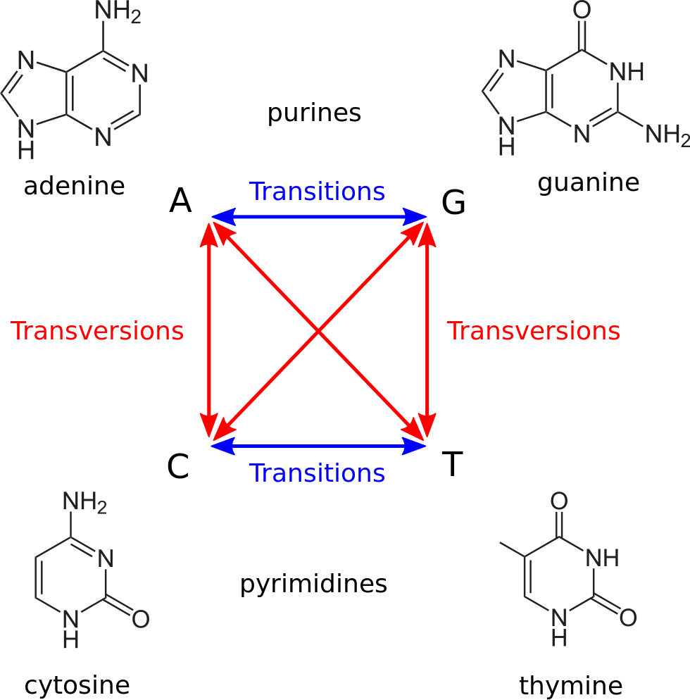 |
| Figure 4. There are two kinds of nucleotide substitutions: Transitions and Transversions. Transitions are substitutions between nucleotides belonging to the same chemical group. For example, a substitution of Adenine, a purine, to Guanine, also a purine, is a transition. Transversions, on the other hand, occur between chemically dissimilar nucleotides. For example, any substitution of a purine to a pyrimidine and vice verse will be a transition. (Image from Wikipedia) |
you can see that there are move ways in which we can have a transversion. Despite this fact transversions are significantly less frequent that transitions. In fact in human the so called Transition/Transversion ratio ($Ts:Tv$) is close to 2 (or even higher in coding regions).
The situation with insertions and deletions (that are often called indels) is similar in that are relatively rare and their rarity increases with size. A single nucleotide indel may occur every 1,000 bases on average, while a two-nucleotide deletion occurs every 3,000 bases and so on (see Montgomery et al. 2013 for a more detailed statistics).
As a result it is simply unrealistic to use “1” is all cases. Instead, we need to penalize rare events more than we penalize frequent, more probable events. Let’s create a penalty matrix to achieve this goal:
Here if two nucleotides match, the penalty is 0. For a transitional substitution we pay $\color{red}2$ and for a transversional we pay $\color{blue}4$. The gap is the most expensive at $\color{orange}8$.
Now, let’s align two sequences:
$\it{X} = \texttt{T A T G T C A T G C}$
and
$\it{Y} = \texttt{T A C G T C A G C}$
First, we need to fill the following dynamic programming matrix:
But now we using penalty matrix generated above to calculate values in each cell. Specifically, before we were using this expression:
but now, we will change it into this:
where $p\texttt{(x,y)}$, $p\texttt{(x,-)}$, and $p\texttt{(-,y)}$ are taken directly from penalty matrix. Let’s start with the first row. In this row we can only fill from the left were we essentially inserting a gap every time. Since the gap penalty is 8 we will get:
Similarly, for the first column we get:
and finally the full matrix:
Drawing a traceback through this matrix will give us:
This corresponds to the following alignment:
T A C G T C A - G C
| | * | | | | * | |
T A T G T C A T G C
The following Python code implements Global alignment approach we have seen above. Note that the first function, exampleCost, can be changed to set different value for the penalty matrix. You can play with it here:
from numpy import zeros

def exampleCost(xc, yc):
    """ Cost function assigning 0 to match, 2 to transition, 4 to
        transversion, and 8 to a gap """
    if xc == yc: return 0 # match
    if xc == '-' or yc == '-': return 8 # gap
    minc, maxc = min(xc, yc), max(xc, yc)
    if minc == 'A' and maxc == 'G': return 2 # transition
    elif minc == 'C' and maxc == 'T': return 2 # transition
    return 4 # transversion

def globalAlignment(x, y, s):
    """ Calculate global alignment value of sequences x and y using
        dynamic programming.  Return global alignment value. """
    D = zeros((len(x)+1, len(y)+1), dtype=int)
    for j in range(1, len(y)+1):
        D[0, j] = D[0, j-1] + s('-', y[j-1])
    for i in range(1, len(x)+1):
        D[i, 0] = D[i-1, 0] + s(x[i-1], '-')
    for i in range(1, len(x)+1):
        for j in range(1, len(y)+1):
            D[i, j] = min(D[i-1, j-1] + s(x[i-1], y[j-1]), # diagonal
                          D[i-1, j  ] + s(x[i-1], '-'),    # vertical
                          D[i  , j-1] + s('-',    y[j-1])) # horizontal
    return D, D[len(x), len(y)]

D, globalAlignmentValue = globalAlignment('TACGTCAGC', 'TATGTCATGC', exampleCost)
print(globalAlignmentValue)
print(D)
Local alignment
Global alignment discussed above works only in cases when we truly expect sequences to match across their entire lengths. In majority of biological application this is rarely the case. For instance, suppose you want to compare two bacterial genomes to figure out if they have matching sequences. Local alignment algorithm helps with this challenge. Surprisingly, it is almost identical to the approaches we used before. So here is our problem:
Sequence 1: ##################################################
                              |||||||||||||||||
Sequence 2:         #################################################
there are two sequences (shown with # characters) and they share a region of high similarity (indicated by vertical lines). How do we find this region? We cannot use global alignment logic here because across the majority of their lengths these sequences are dissimilar.
To approach this problem we will change our penalty strategy. Instead of giving a high value for each mismatch we will instead give negative penalties. Only matches get positive rewards. Here is an example of such scoring matrix (as opposed to the penalty matrix we’ve used before):
Our scoring logic will also change:
We are now looking for maximum and use 0 to prevent having negative values in the matrix. This also implies that the first row and column will now be filled with zeros. Let apply this to two sequences:
Now, let’s align two sequences:
$\texttt{T A T A T G C G G C G T T T}$
and
$\texttt{G G T A T G C T G G C G C T A}$
Dynamic programming matrix with initialized first row and column will look like this:
Filling it completely will yield the following matrix. Note that clues to where the local alignment may be are given off by positive numbers in the sea of 0s:
To identify to boundary of the local alignment we need to identify the cell with the highest value. This cell has value of $\color{red}{12}$ and is highlighted above. Using traceback procedure we will find:
This corresponds to the best local alignment between the two sequences:
 T A T A T G C - G G C G T T T
     | | | | | * | | | |
 G G T A T G C T G G C G C T A
Here is a Python representation of this approach:
import numpy

def exampleCost(xc, yc):
    ''' Cost function: 2 to match, -6 to gap, -4 to mismatch '''
    if xc == yc: return 2 # match
    if xc == '-' or yc == '-': return -6 # gap
    return -4

def smithWaterman(x, y, s):
    ''' Calculate local alignment values of sequences x and y using
        dynamic programming.  Return maximal local alignment value. '''
    V = numpy.zeros((len(x)+1, len(y)+1), dtype=int)
    for i in range(1, len(x)+1):
        for j in range(1, len(y)+1):
            V[i, j] = max(V[i-1, j-1] + s(x[i-1], y[j-1]), # diagonal
                          V[i-1, j  ] + s(x[i-1], '-'),    # vertical
                          V[i  , j-1] + s('-',    y[j-1]), # horizontal
                          0)                               # empty
    argmax = numpy.where(V == V.max())
    return V, int(V[argmax])

def traceback(V, x, y, s):
    """ Trace back from given cell in local-alignment matrix V """
    # get i, j for maximal cell
    i, j = numpy.unravel_index(numpy.argmax(V), V.shape)
    xscript, alx, aly, alm = [], [], [], []
    while (i > 0 or j > 0) and V[i, j] != 0:
        diag, vert, horz = 0, 0, 0
        if i > 0 and j > 0:
            diag = V[i-1, j-1] + s(x[i-1], y[j-1])
        if i > 0:
            vert = V[i-1, j] + s(x[i-1], '-')
        if j > 0:
            horz = V[i, j-1] + s('-', y[j-1])
        if diag >= vert and diag >= horz:
            match = x[i-1] == y[j-1]
            xscript.append('M' if match else 'R')
            alm.append('|' if match else ' ')
            alx.append(x[i-1]); aly.append(y[j-1])
            i -= 1; j -= 1
        elif vert >= horz:
            xscript.append('D')
            alx.append(x[i-1]); aly.append('-'); alm.append(' ')
            i -= 1
        else:
            xscript.append('I')
            aly.append(y[j-1]); alx.append('-'); alm.append(' ')
            j -= 1
    xscript = (''.join(xscript))[::-1]
    alignment = '\n'.join(map(lambda x: ''.join(x), [alx[::-1], alm[::-1], aly[::-1]]))
    return xscript, alignment

x, y = 'GGTATGCTGGCGCTA', 'TATATGCGGCGTTT'
V, best = smithWaterman(x, y, exampleCost)
print(V)
print("Best score=%d, in cell %s" % (best, numpy.unravel_index(numpy.argmax(V), V.shape)))
print(traceback(V, x, y, exampleCost)[1])
This algorithm was developed by Temple Smith and Michael Waterman in 1981. This is why it is most often called Smith Waterman local alignment algorithm.
Homework
- Modify the last code snippet of this lecture (local alignment code) to output seaborn heatmap visualization of the matrix. Use any color scheme that is not default.
- Produce similar heatmap using matrix visualization function of
toyplot. To do this you will need to installtoyplotinto your notebook usingpip.