Analysis of RNA I: Molecular Biology of SARS-COV-2
SARS-COV-2 COVID-19 RNAseq
A quick overview of coronavirus molecular biology
Given the current situation we will continue this class using SARS-COV-2 as example for all further analyses. So far we have covered variant calling and genome assembly. Next we will be looking into RNAseq. Since SARS-COV-2 is a positive strand RNA virus that pretends to be a typical human transcript, it is a great system to learn about RNAseq. But first we need to learn about the coronavirus molecular biology. This is what we will do in this lecture.
The following summary is based on these publications:
Genome organization
All coronaviruses contain non-segmented positive strand RNA genome approx. 30 kb in length. It is invariably 5’-leader-UTR-replicase-S-E-M-N-3’UTR-poly(A). In addition, it contains a variety of accessory proteins interspersed throughout the genome (see Fig. below).
Genomic organization of representative α, β, and γ CoVs. An illustration of the MHV genome is depicted at the top. The expanded regions below show the structural and accessory proteins in the 3′ regions of the HCoV-229E, MHV, SARS-CoV, MERS-CoV and IBV. Size of the genome and individual genes are approximated using the legend at the top of the diagram but are not drawn to scale. HCoV-229E human coronavirus 229E, MHV mouse hepatitis virus, SARS-CoV severe acute respiratory syndrome coronavirus, MERS-CoV Middle East respiratory syndrome coronavirus, IBV infectious bronchitis virus. (From Fehr and Perlman:2015)
The long replicase gene encodes a number of non-structural proteins (nsps) and occupies 2⁄3 or the genome. Because of -1 ribosomal frameshifting within ORFab approx. in 25% of the cases polyprotein pp1ab is produced in place of pp1a. pp1a encodes 11 nsps while pp1ab encodes 15.

Coronavirus genome structure and gene expression. (a) Coronavirus genome structure. The upper scheme represents the TGEV genome. Labels indicate gene names; L corresponds to the leader sequence. Also represented are the nsps derived from processing of the pp1a and pp1ab polyproteins. PLP1, PLP2, and 3CL protease sites are depicted as inverted triangles with the corresponding color code of each protease. Dark gray rectangles represent transmembrane domains, and light gray rectangles indicate other functional domains. (b) Coronavirus genome strategy of sgmRNA expression. The upper scheme represents the TGEV genome. Short lines represent the nested set of sgmRNAs, each containing a common leader sequence (black) and a specific gene to be translated (dark gray). © Key elements in coronavirus transcription. A TRS precedes each gene (TRS-B) and includes the core sequence (CS-B) and variable 5′ and 3′ flanking sequences. The TRS of the leader (TRS-L), containing the core sequence (CS-L), is present at the 5′ end of the genome, in an exposed location (orange box in the TRS-L loop). Discontinuous transcription occurs during the synthesis of the negative-strand RNA (light blue), when the copy of the TRS-B hybridizes with the TRS-L. Dotted lines indicate the complementarity between positive-strand and negative-strand RNA sequences. Abbreviations: EndoU, endonuclease; ExoN, exonuclease; HEL, helicase; MTase, methyltransferase (green, N7-methyltransferase; dark purple, 2′-O-methyltransferase); nsp, nonstructural protein; PLP, papain-like protease; RdRp, RNA-dependent RNA polymerase; sgmRNA, subgenomic RNA; TGEV, transmissible gastroenteritis virus; TRS, transcription-regulating sequence; UTR, untranslated region. (From Sola:2015).
Virion structure
Coronovirus is a spherical particle approx. 125 nm in diameter. It is covered with S-protein projections giving it an appearance of solar corona - hence the term coronavirus. Inside the envelope is nucleocapsid that has helical symmetry far more typical of (-)-strand RNA viruses. There are four main structure proteins: spike (S), membrane (M), envelope (E), and nucleocapsid (N).

Schematic of the coronavirus virion, with the minimal set of structural proteins (From Masters:2006).
Mature S protein is trimer of two subunits: S1 and S2. The two subunits are produced from a single S-precursor by host proteases (see Kirchdoerfer:2016; this however is not the case for all coronaviruses such as SARS-CoV). S1 forms the receptor-binding domain, while S2 forms the stalk.
M protein is the most abundant structural components of the virion and determines its shape. It possibly exists as a dimer.
E protein is least abundant protein of the capsid and possess ion channel activity. In facilitates assembly and release of the virus. In SARS-CoV it is not required for replication but is essential for pathogenesis.
N proteins forms the nucleocapsid. It N- and C-terminal domains are capable of RNA binding. Specifically it binds to transcription regulatory sequences and the genomic packaging signal. It also binds to nsp3 and M protein possible tethering viral genome and replicase-transcriptase complex.
Entering the cell
Virion attaches to the cells as a result of interaction between S-protein and a cellular receptor. In case of SARS-CoV-2 (as is in SARS-CoV) angiotensin converting enzyme 2 (ACE2) serves as the receptor binding to C-terminal portion of S1 domain. After receptor binding S protein is cleaved at two sites within the S2 subdomain. The first cleavage separates receptor-binding domain of S from membrane fusion domain. The second cleavage (at S2’) exposes the fusion peptide. The SARS-CoV-2 is different from SARS-CoV in that it contains a furin cleavage site that is processed during viral maturation within endoplasmatic reticulum (ER; see Walls:2020). The fusion peptide inserts into the cellular membrane and triggers joining on the two heptad regions with S2 forming antiparallel six-helix bundle resulting in fusion and release of the genome into the cytoplasm.
Replication
The above figure shows that in addition to the full length (+)-strand genome there is a number of (+)-strand subgenomic RNAs corresponding to 3’-end of the complete viral sequence. All of these subgenomic RNAs (sgRNAs) share the same leader sequence that is present only once at the extreme 5’-end of the viral genome. These RNAs are produced via discontinuous RNA synthesis when the RNA-dependent RNA-polymerase (RdRp) switches template:
Model for the formation of genome high-order structures regulating N gene transcription. The upper linear scheme represents the coronavirus genome. The red line indicates the leader sequence in the 5′ end of the genome. The hairpin indicates the TRS-L. The gray line with arrowheads represents the nascent negative-sense RNA. The curved blue arrow indicates the template switch to the leader sequence during discontinuous transcription. The orange line represents the copy of the leader added to the nascent RNA after the template switch. The RNA-RNA interactions between the pE (nucleotides 26894 to 26903) and dE (nucleotides 26454 to 26463) and between the B-M in the active domain (nucleotides 26412 to 26421) and the cB-M in the 5′ end of the genome (nucleotides 477 to 486) are represented by solid lines. Dotted lines indicate the complementarity between positive-strand and negative-strand RNA sequences. Abbreviations: AD, active domain secondary structure prediction; B-M, B motif; cB-M, complementary copy of the B-M; cCS-N, complementary copy of the CS-N; CS-L, conserved core sequence of the leader; CS-N, conserved core sequence of the N gene; dE, distal element; pE, proximal element; TRS-L, transcription-regulating sequence of the leader (From Sola:2015).
Furthermore Sola:2015) suggest propose the coronavirus transcription model in which transcription initiation complex forms at the 3’-end of (+)-strand genomic RNA:

Three-step model of coronavirus transcription. (1) Complex formation. Proteins binding transcription-regulating sequences are represented by ellipsoids, the leader sequence is indicated with a red bar, and core sequences are indicated with orange boxes. (2) Base-pairing scanning. Negative-strand RNA is shown in light blue; the transcription complex is represented by a hexagon. Vertical lines indicate complementarity between the genomic RNA and the nascent negative strand. (3) Template switch. Due to the complementarity between the newly synthesized negative-strand RNA and the transcription-regulating sequence of the leader, template switch to the leader is made by the transcription complex to complete the copy of the leader sequence (From Sola:2015).
So what can we do?
Given this information we ask the following questions:
- Can we reconstruct individual transcripts given the SARS-CoV data?
- Can we observe and confirm the ribosomal frameshifting?
- Can we identify secondary structures within SARS-CoV RNAs?
- …. Suggest your own question ….
Yes, we can do all these things. We will start with question I: transcript reconstruction.
Reference-based RNAseq
This tutorial is inspired by an exceptional RNAseq course at the Weill Cornell Medical College compiled by Friederike Dündar, Luce Skrabanek, and Paul Zumbo and by tutorials produced by Björn Grüning (@bgruening) for Freiburg Galaxy instance. Much of Galaxy-related features described in this section have been developed by Björn Grüning (@bgruening) and configured by Dave Bouvier (@davebx).
RNAseq can be roughly divided into two “types”:
- Reference genome-based - an assembled genome exists for a species for which an RNAseq experiment is performed. It allows reads to be aligned against the reference genome and significantly improves our ability to reconstruct transcripts. This category would obviously include humans and most model organisms but excludes the majority of truly biologically intereting species (e.g., Hyacinth macaw);
- Reference genome-free - no genome assembly for the species of interest is available. In this case one would need to assemble the reads into transcripts using de novo approaches. This type of RNAseq is as much of an art as well as science because assembly is heavily parameter-dependent and difficult to do well.
In this lesson we will focus on the Reference genome-based type of RNA seq.
Experimental procedures affect downstream analyses
The Everything’s connected slide by Dündar et al. (2015) explains the overall idea:

There is a variety of ways in which RNA is treated during its conversion to cDNA and eventual preparation of sequencing libraries. In general the experimental workflow includes the following steps:
- RNA purification;
- Reverse transcription using Reverse Transcriptase (RT), which produces the first strand of cDNA (“c” stands for complimentary);
- Second strand synthesis using DNA polymerase;
- Library preparation for sequencing.
In listing these basic steps we are ignoring a vast amount of details such as, for example, normalization strategies and procedures needed to deal with rare RNAs or degraded samples (see Adiconis:2013). Yet, there are two important experimental considerations that would effect the ways in which one analyses data and interprets the results. These are:
- Priming for the first cDNA strand synthesis;
- Stranded versus Non-stranded libraries.
Priming for the first strand synthesis
Reverse Transcriptase (RT) requires a primer. One can leverage the fact that the majority of processed mRNAs are polyadenylated and use oligo-dT primer to (mostly) restrict cDNA synthesis to fully processed mRNAs. Alternatively one can use a mix of random oligonucleotides to prime RT at a multitude of internal sites irrespective of RNA type and maturation status:
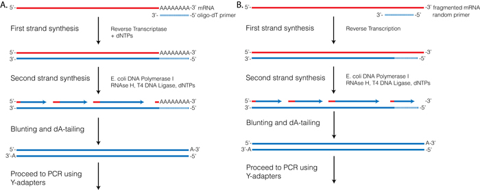 |
| Oligo-dT vs. random priming |
| Oligo-dT (A) and random priming (B) |
Depending on the choice of the approach one would have different types of RNAs included in the final sequencing outcome. For example, if one attempts to study RNAs that are not polyadenylated or not fully processed, it would be unwise to use oligo-dT priming approach.
Strand-specific RNAseq
RNAs that are typically targeted in RNAseq experiments are single stranded (e.g., mRNAs) and thus have polarity (5’ and 3’ ends that are functionally distinct):
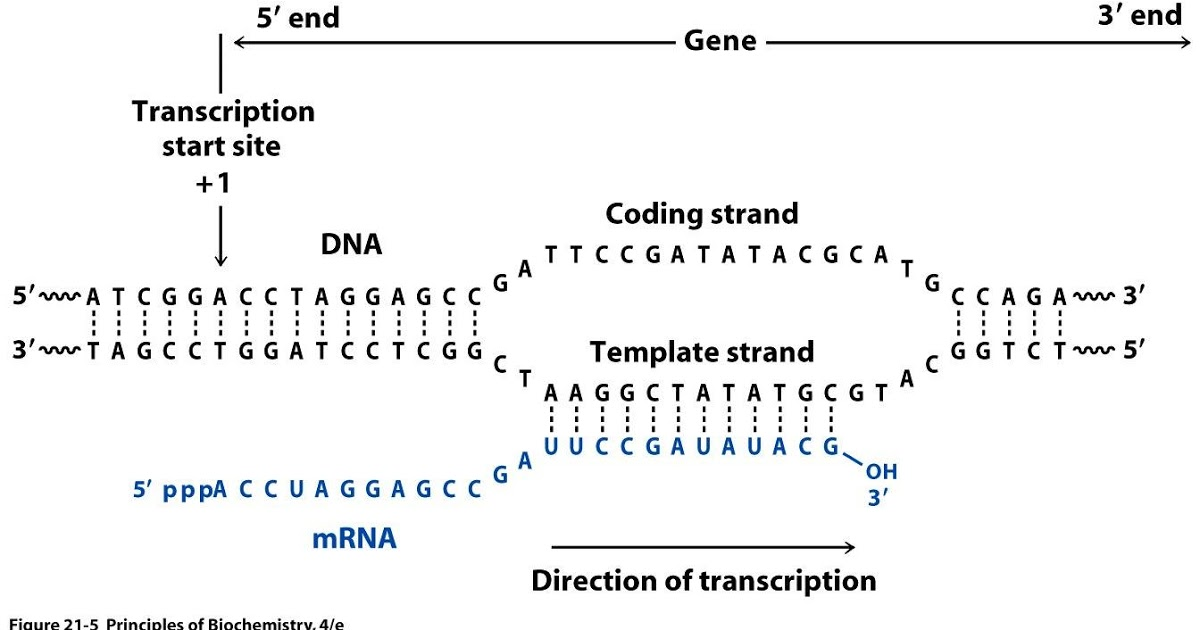 |
| Relationship between DNA and RNA orientation |
During a typical RNAseq experiment the information about strandedness is lost after both strands of cDNA are synthesized, size selected, and converted into sequencing library. However, this information can be quite useful for various aspects of RNAseq analysis such as transcript reconstruction and quantification. There is a number of methods for creating so called stranded RNAseq libraries that preserve the strand information (for an excellent overview see Levin et al. 2010):
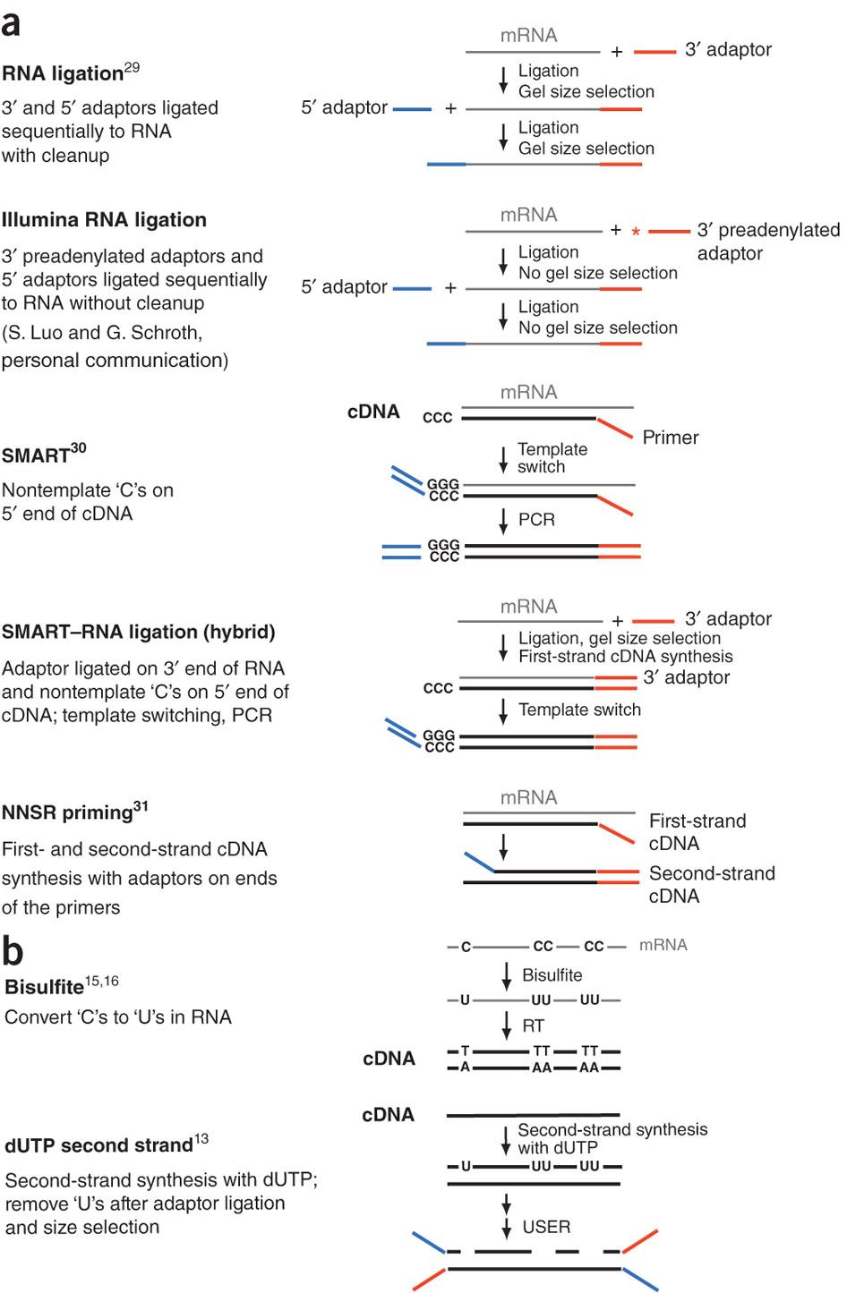 |
| Generation of stranded RNAseq libraries. Different types of stranded library generation protocols from Levin:2010 |
Depending on the approach and whether one performs single- or paired-end sequencing there are multiple possibilities on how to interpret the results of mapping of these reads onto genome/transcriptome:
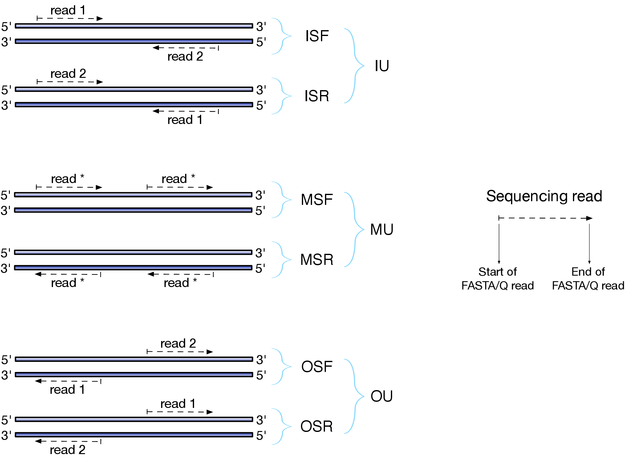 |
| Effects of RNAseq library types |
| Image and description below is from Sailfish documentation |
The relative orientation of the reads is only relevant if the library is pair-ended. The possible options are:
- I = inward;
- O = outward;
- M = matching (co-directional).
Library can be stranded (S) or unstranded (U). If this library is stranded than depending on the protocols reads (single reads or forward reads in a paired-end run) may originate from:
- F = read 1 in paired-end sequencing or single-end read is derived from the Forward strand;
- R = read 1 in paired-end sequencing or single-end read is derived from the Reverse strand.
So by combining the relative orientation of reads is I, O, or M (if reads are paired), strandedness or the library (S or U), and whether the reads originate from forward and reverse strand (F or R) there can be quite a number of possibilities:
- IU - (an unstranded paired-end library where the reads face each other)
- SF - (a stranded single-end protocol where the reads come from the forward strand)
- OSR - (a stranded paired-end protocol where the reads face away from each other, read1 comes from reverse strand and read2 comes from the forward strand). and so on…
However, in practice, if you use Illumina paired-end RNAseq protocols you are unlikely to uncover many of these possibilities. You will either deal with:
- unstranded RNAseq data (IU type from above. Also called fr-unstranded in TopHat/Cufflinks jargon);
- stranded RNAseq data produced with Illumina TrueSeq RNAseq kits and dUTP tagging (ISR type from above or fr-firststrand in TopHat/Cufflinks nomenclature).
The implication of stranded RNAseq is that you can distinguish whether the reads are derived from forward- or reverse-encoded transcripts:
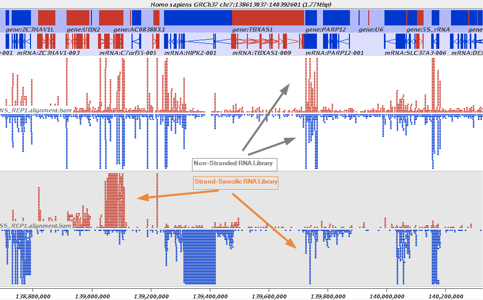 |
| Stranded RNAseq data look like this This example contrasts unstranded and stranded RNAseq experiments. Red transcripts are from + strand and blue are from - strand. In stranded example reads are clearly stratified between the two strands. A small number of reads from opposite strand may represent anti-sense transcription. The image from GATC Biotech. |
Replicates: Biological or Technical and how many?
An RNAseq experiment without a sufficient number of replicates will be a waste of money. Replicates are essential to be able to correct for variation due to differences within/among organisms, cells, sequencing machines, library preparation protocols and numerous other potential factors. There are two types of replicates (as described by Dündar:2015):
Technical replicates can be defined as different library preparations from the same RNA sample. They should account for batch effects from the library preparation such as reverse transcription and PCR amplification. To avoid possible lane effects (e.g., differences in the sample loading, cluster amplification, and efficiency of the sequencing reaction), it is good practice to multiplex the same sample over different lanes of the same flowcell. In most cases, technical variability introduced by the sequencing protocol is quite low and well controlled.
Biological replicates. There is an on-going debate over what kinds of samples represent true biological replicates. Obviously, the variability between different samples will be greater between RNA extracted from two unrelated humans than between RNA extracted from two different batches of the same cell line. In the latter case, most of the variation that will eventually be detected was probably introduced by the experimenter (e.g., slightly differing media and plating conditions). Nevertheless, this is variation the researcher is typically not interested in assessing, therefore the ENCODE consortium defines biological replicates as RNA from an independent growth of cells/tissue (ENCODE 2011).
The number of replicates should be as high as practically possible. Most RNAseq experiments include three replicates and some have as many as 12 (see Schurch et al. 2015).
Read mapping
After sequencing is performed you have a collection of sequencing reads for each sample/replicate. In a reference-based RNAseq experiment these need to be mapped against the genome. Because in the case of eukaryotic transcriptome most reads originate from processed mRNAs lacking exons, they cannot be simply mapped back to the genome. Instead they can be separated into two categories:
- Reads that map entirely within exons
- Reads that cannot be mapped within an exon across their entire length because they span two or more exons
Spliced mappers have been developed to efficiently map transcript-derived reads against genome.
TopHat, TopHat2, and HiSat
Tophat was one of the first tools designed specifically to address this problem by identifying potential exons using reads that do map to the genome, generating possible splices between neighboring exons, and comparing reads that did not initially map to the genome agaisnt these in silico created junctions:
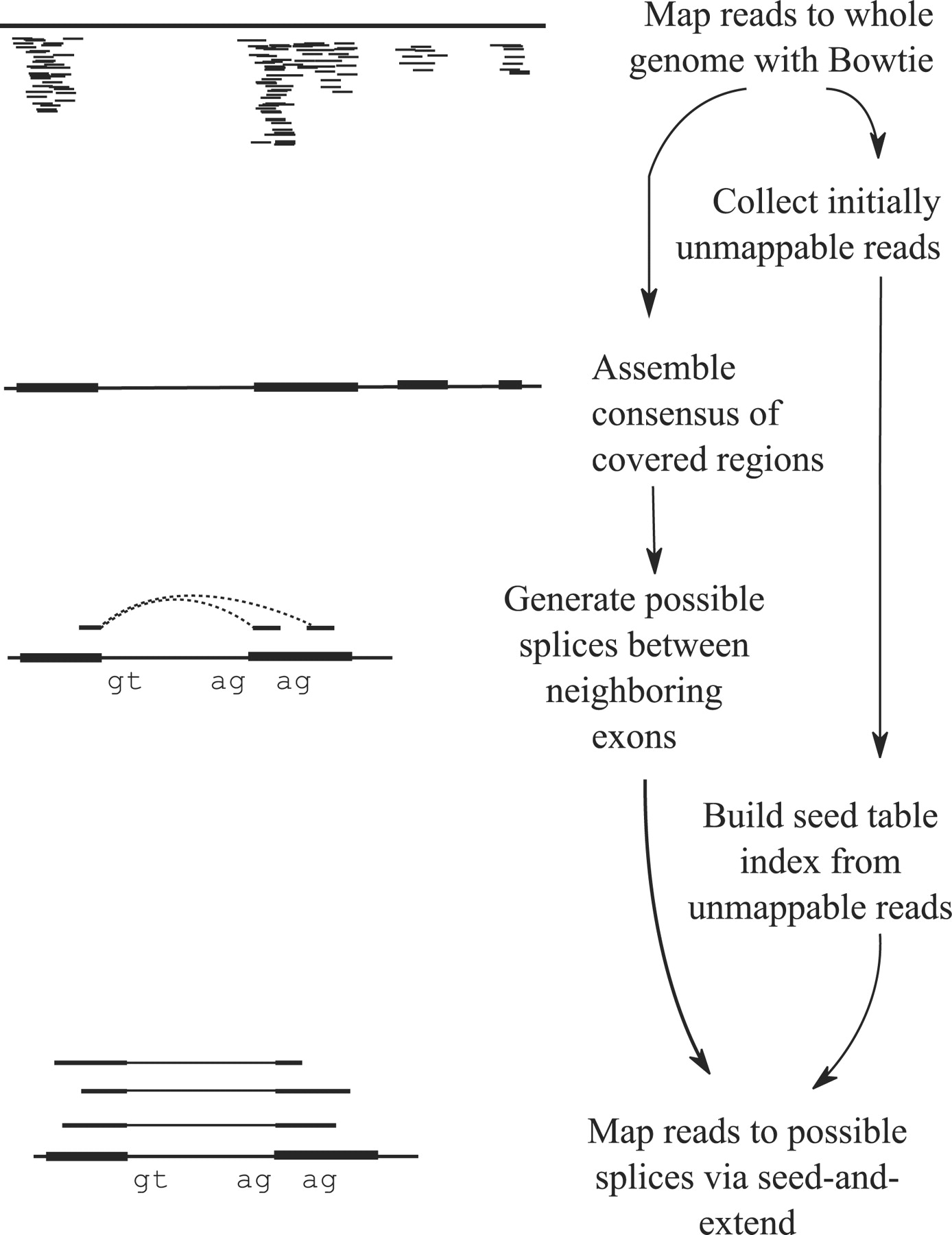 |
| TopHat and TopHat2: Mapping RNAseq regions to genome. In TopHat reads are mapped against the genome and are separated into two categories: (1) those that map, and (2) those that initially unmapped (IUM). “Piles” of reads representing potential exons are extended in search of potential donor/acceptor splice sites and potential splice junctions are reconstructed. IUMs are then mapped to these junctions. Image from Trapnell:2009. |
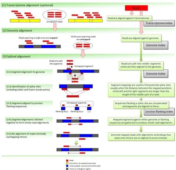 |
| TopHat has been subsequently improved with the development of TopHat2. Image from Kim:2012 summarizes steps involved in aligning of RNAseq reads with TopHat2. |
To further optimize and speed up spliced read alignment Kim at al. 2015 developed HISAT. It uses a set of FM-indices consisting one global genome-wide index and a collection of ~48,000 local overlapping 42 kb indices (~55,000 56 kb indices in HiSat2). This allows to find initial seed locations for potential read alignments in the genome using global index and to rapidly refine these alignments using a corresponding local index:
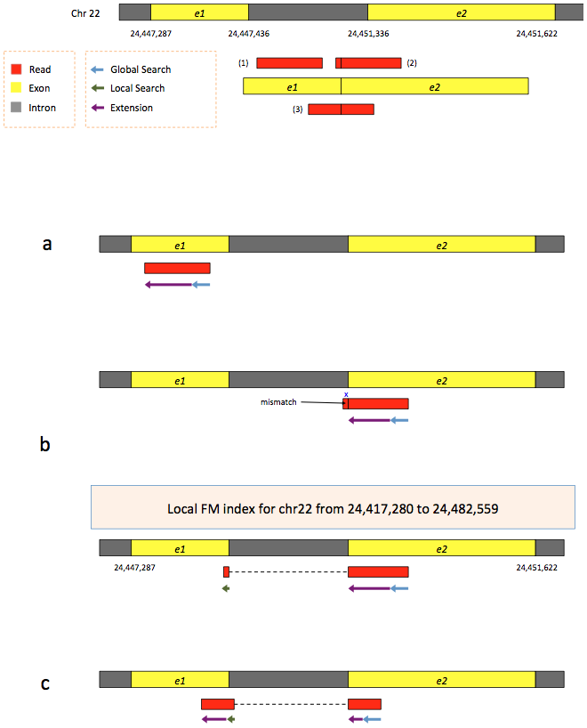 |
| Hierarchical Graph FM index in HiSat/HiSat2. A part of the read (blue arrow) is first mapped to the genome using the global FM index. The HiSat then tries to extend the alignment directly utilizing the genome sequence (violet arrow). In (a) it succeeds and this read aligned as it completely resides within an exon. In (b) the extension hits a mismatch. Now HiSat takes advantage of the local FM index overlapping this location to find the appropriate matching for the remainder of this read (green arrow). The (c) shows a combination these two strategies: the beginning of the read is mapped using global FM index (blue arrow), extended until it reaches the end of the exon (violet arrow), mapped using local FM index (green arrow) and extended again (violet arrow). Image from Kim:2015 |
STAR mapper
STAR aligner is a fast alternative for mapping RNAseq reads against genome utilizing uncompressed suffix array. It operates in two stages. In the first stage it performs seed search:
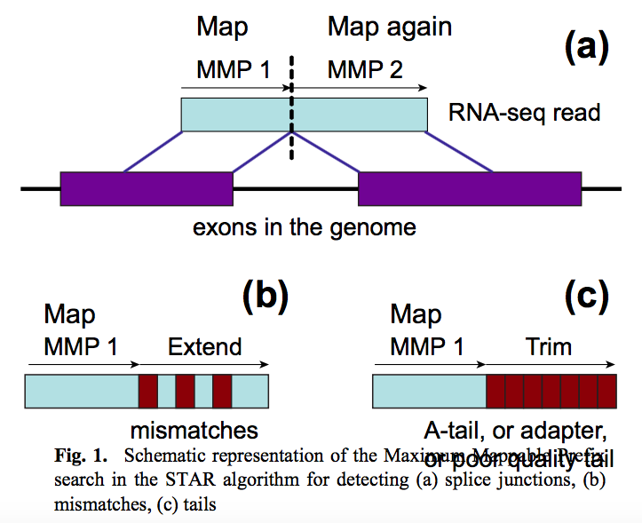 |
| STAR’s seed search. Here a read is split between two consecutive exons. STAR starts to look for a maximum mappable prefix (MMP) from the beginning of the read until it can no longer match continuously. After this point it starts to MMP for the unmatched portion of the read (a). In the case of mismatches (b) and unalignable regions (c) MMPs serve as anchors from which to extend alignments. Image from Dobin:2013. |
At the second stage STAR stitches MMPs to generate read-level alignments that (contrary to MMPs) can contain mismatches and indels. A scoring scheme is used to evaluate and prioritize stitching combinations and to evaluate reads that map to multiple locations. STAR is extremely fast but requires a substantial amount of RAM to run efficiently.
Transcript reconstruction
The previous step - mapping - assigns RNAseq reads to genomic locations and identifies splice junctions from reads that originate from different exons. At transcript reconstruction step this information is taken further in attempt to build transcript models. There is a number of tools for performing this task. A benchmarking paper by Hayer:2015 attempted to compare performance of existing approaches with one of the outcomes shown below:
 |
| Comparison of transcript reconsruction approaches. Here recall (the number of correctly constructed forms divided by the total number of real forms) versus precision (true positives divided by the sum of true positives and false positives) are plotted for seven transcript assemblers tested on two simulated datasets: EnsemblPerfect and EnsemblRealistic. The shaded region is indicating suboptimal performance (i.e., the white, unshaded region is “good”). The figure is from Hayer:2015. |
Based on these results Cufflinks and StringTie have satisfactory performence. The following discussion is based on inner workings of StringTie.
Transcriptome assembly with StringTie
StringTie assembles transcripts from spliced read alignemnts produced by tools such as STAR, TopHat, or HISAT and simultaneously estimates their abundances using counts of reads assigned to each transcript. The following images illustrates details of StringTie workflow:
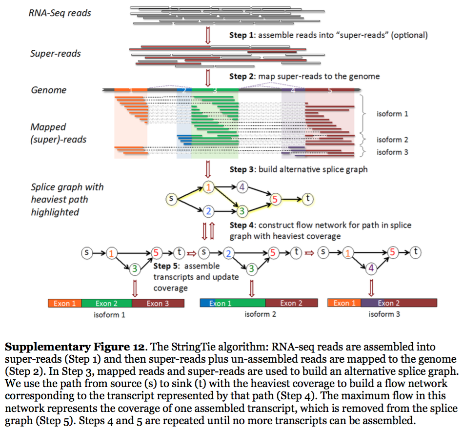 |
| StringTie workflow. Image from Pertea:2015 |
In essence StringTie builds an alternative splice graph from overlapping reads in a given locus. In such a graph nodes correspond to exons (or, rather, contiguous regions of genome covered by reads; colored regions on the figure above), while edges are represented by reads connecting these exons. Next, it identifies a path within the splice graph that has the highest weight (largest number of reads on edges). Such path would correspond to an assembled transcript at this iteration of the algorithm. Because the edge weight is equal to the number of the reads StringTie estimates the coverage level for this transcript (see below) which can be used to estimate the transcript’s abundance. Reads that are associated with the transcript that was just assembled are then removed and the graph is updated to perform the next iteration of the algorithm.
Transcript quantification
Transcriptome quantification attempts to estimate expression levels of individuals transcripts. This is performed by assigning RNAseq reads to transcripts, counting, and normalization.
Assigning reads to transcripts
To associate reads with transcripts they (the reads) need to be aligned to the transcriptome. Tools like Cufflinks and StringTie reconstruct transcripts from spliced read alignments generated by other programs (TopHat, HISAT, STAR), so they already have the information about which reads belong to each reconstructed transcript. Other tools such as Sailfish, Kallisto, and Salmon perform lightweight alignment of RNAseq reads against existing transcriptome sequences. The goal of lightweight alignment is to quickly distribute the reads across transcripts they likely originate from without worrying too much about producing high quality alignments. The upside of this is that the entire procedure can be performed very quickly. The downside is that these tools require high quality transcriptome as input, which is not a problem if you work with humans or mice, but is a problem if you are studying Hyacinth macaw or any other brilliantly colored creature.
Lightweight alignment
Sailfish has been initially designed to utilize k-mer matching for finding association between reads and corresponding transcripts:
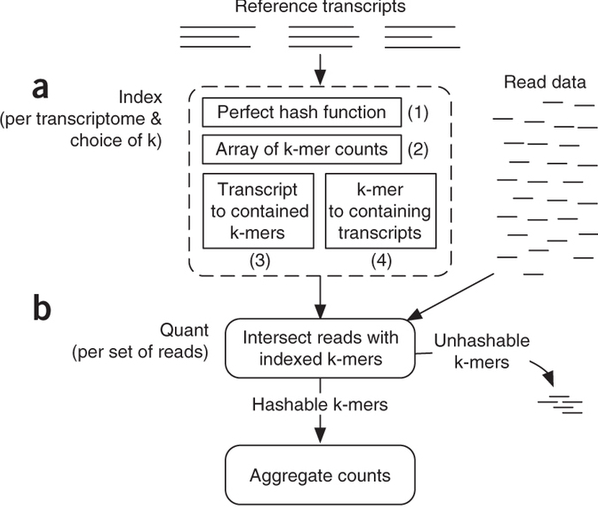 |
| Assigning reads to transcripts: Sailfish. Sailfish indexes input transcriptome for a fixed k-mer length and compares k-mers derived from RNAseq reads against this index. Image from Patro:2014 |
The current version of Sailfish uses quasi-alignment to extend exact matches found with k-mers:
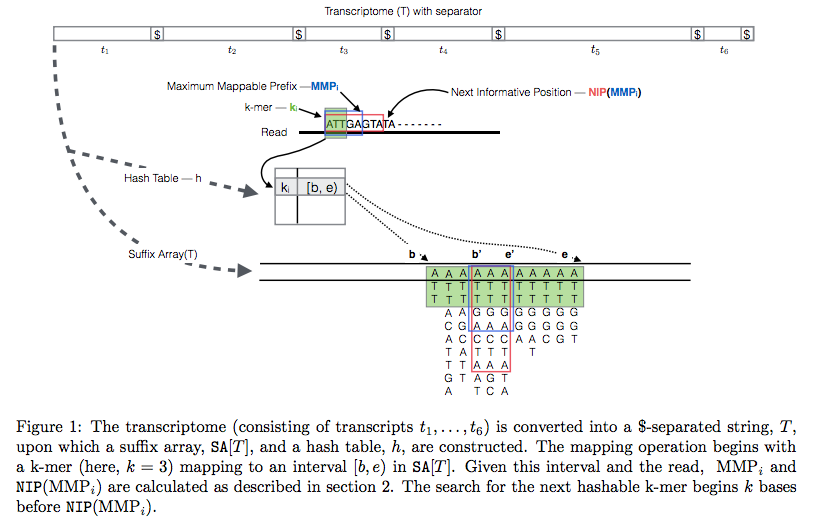 |
Quasi-alignment of reads in Sailfish. In Sailfish version 0.7.0 and up transcriptome is concatenated into a single sequence using $ separators from which a suffix array and a hash table are constructed. A k-mer from an RNAseq read (green) is looked up in the hash table, which immediately gives its position in the suffix array allowing to extend the march as described in the legend and the paper. Image from Srivastava:2015 |
Kallisto also utilizes k-mer matching but uses a different data structure. It constructs a De Bruijn graph from transcriptome input (pane b of the figure below). This graph is different from De Bruijn graphs used for genome assembly in that its nodes are k-mers and transcripts correspond to paths through the graph. To accommodate multiple transcripts that can lay along the same path (or sub-path) the paths are “colored” with each transcript given a distinct “color” (in genome assembly the graph is built from the reads and nodes usually correspond to overlaps between k-mers forming incoming and outgoing edges). Non-branching sections of the graph that have identical coloring are “glued” into contigs. Finally a hash table is built that stores the position of each transcriptome k-mer within the graph:
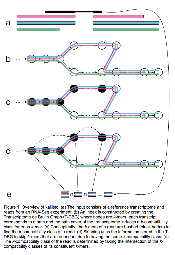 |
| Assigning reads to transcripts: Kallisto. Here a black read is being associated with a set consisting of red, blue, and green transcripts (a). First, a graph is built from transcriptome (b). Next, by finding common k-mers between the read and the graph the read is “threaded” along a path (c and d). The colors along that path would indicate which transcripts it is likely derived from. Specifically, this is done by taking intersection of “colors” (c). It this case the read is assigned to two transcripts: red and blue. Image from Bray:2015 |
Salmon does not use k-mer matching approach. Instead it creates bwa-like FM-index and uses it to finds chains of Maximal Exact Matches (MEMs) and Super Maximal Exact Matches (SMEMs) between a read and the transcriptome.
Patro:2015 define a MEM as “a substring that is shared by the query (read) and reference (transcript) that cannot be extended in either direction without introducing a mismatch”. Similraly, a SMEM is defined as a “MEM that is not contained within any other MEM on the query.” One of the advantages of utilizing the FM-index is that a new index does not need to re-generated for a search with different set of parameters. In the case of Sailfish and Kallisto an index is dependent on k-mer length and has to be recomputed every time the k is changed. The overall schematics of Salmon operation is as follows:
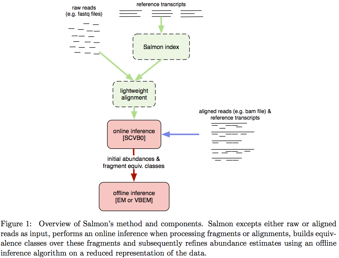 |
| Assigning reads to transcripts: Salmon. Image from Patro:2015 |
Estimating transcript levels
Once reads are apportioned across individual transcripts they can be quantified. There are several approaches for quantification.
Flow networks
StringTie, which performs assembly and quantification simultaneously converts splice graph into a flow network for which it solves the maximum flow problem. The maximum flow is such network represents the expression level for a given transcript:
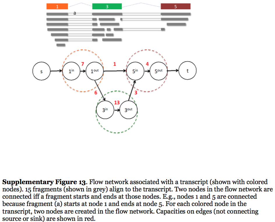 |
| StringTie flow network. Here each exon node from the splice graph is split into in and out nodes connected with an edge weighted by the number of reads corresponding to that exon. For example, the first exon is covered by seven reads and so the edge between 1-in and 1-out has a weight of 7. Expression level would correspond to the maximum flow through a path representing a given transcript. Image from Pertea:2015 |
Expectation Maximization
The Expectation/Maximization framework (EM) is utilized in a number of tools such as eXpress and more recently Sailfish, Kallisto, and Salmon (As an alternative strategy Salmon also utilizes variational Bayesian method. The principle of EM is nicely illustrated by Lior Pachter in his transcript quantification review. Suppose, as shown on the image below, there are three transcripts (green, red, and blue). There are five reads associated with these transcripts. One read (d) is unique to the red transcript, while others correspond to two (b, c, e) or three (a) transcripts. The EM is an iterative procedure. In the first round transcript abundances are initialized as equal (0.33 each as there are three transcripts) and during expectation reads are apportioned across transcripts based on these abundances. Next, during maximization step transcript abundances are re-calculated as follow. For red transcript we sum up fraction of each read as 0.33 + 0 + 0.5 + 1 + 0.5 for reads a, b, c, d, and e, respectively. We now divide this by the sum of read allocations for each transcript as 2.33 + 1.33 + 1.33 for red, green, and blue transcripts respectively. For all three transcript calculation will look like this:
During next expectation stage read are re-apportioned across transcripts and the procedure is repeated until convergence:
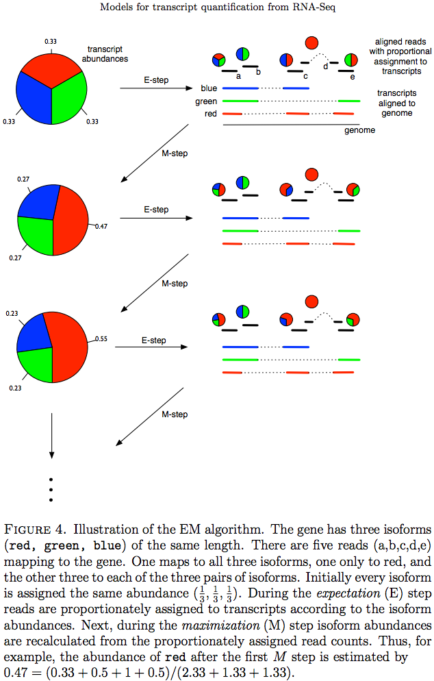 |
| Expectation Maximization (EM). Image from Pacher:2011 |
Understanding quantification metrics
As we’ve seen above quantification for a transcript is estimated using the number of associated reads. Yet the count is not a very good measure as it will be severely biased by multiple factors such as, for example, transcript length. Thus these counts need to be normalized. Normalization strategies can be roughly divided into two groups:
- Normalization for comparison within a single sample;
- Normalization for comparison among multiple samples/conditions.
In their tutorial Dündar et al. have compiled a table summarizing various metrics. Below is description of normalization technique for within sample comparisons (between sample comparison can be found in the next section on differential expression analysis):
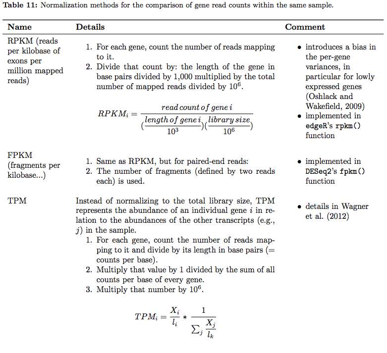 |
| RNAseq normalization metrics: Within sample comparisons. Table from Dündar et al. 2015 |
In addition, an excellent overview of these metrics can be found here.
⚠ You should NEVER EVER use RPKM, FPKM, or TPM to compare expression levels across samples. These are RELATIVE measures! Consider yourself warned!
Homework
Identify reasonable starting here: