NumPy

Mar 2, 2020
python numpy

Prep

Point your browser to http://colab.research.google.com
Open notebook 2020/ipynb/numpy.ipynb from https://github.com/nekrut/BMMB554

Numpy: Operations with multidimensional data

This notebook is based (with some modifications) on a NumPy tutorial by J.R. Johansson

# Import MatPlotlib so we can look at some pretty plots
# The reson for doing this will become clear in out MatPlotLib lecture next week
%matplotlib inline
import matplotlib.pyplot as plt

Introduction

The numpy package (module) is used in almost all numerical computation using Python. It is a package that provide high-performance vector, matrix and higher-dimensional data structures for Python. It is implemented in C and Fortran so when calculations are vectorized (formulated with vectors and matrices), performance is very good.

To use numpy you need to import the module, using for example:

from numpy import *

In the numpy package the terminology used for vectors, matrices and higher-dimensional data sets is array.

Creating numpy arrays

There are a number of ways to initialize new numpy arrays, for example from

a Python list or tuples
using functions that are dedicated to generating numpy arrays, such as arange, linspace, etc.
reading data from files

From lists

For example, to create new vector and matrix arrays from Python lists we can use the numpy.array function.

# a vector: the argument to the array function is a Python list
vector = array([1,2,3,4])

vector

array([1, 2, 3, 4])

# a matrix: the argument to the array function is a nested Python list
matrix = array([[1, 2], [3, 4]])

matrix

array([[1, 2],
       [3, 4]])

The v and M objects are both of the type ndarray that the numpy module provides:

type(vector), type(matrix)

(numpy.ndarray, numpy.ndarray)

The difference between the v and M arrays is only their shapes. We can get information about the shape of an array by using the ndarray.shape property:

vector.shape

(4,)

matrix.shape

(2, 2)

The number of elements in the array is available through the ndarray.size property:

matrix.size

Equivalently, we could use the function numpy.shape and numpy.size:

shape(matrix)

(2, 2)

size(matrix)

So far the numpy.ndarray looks awefully much like a Python list (or nested list). Why not simply use Python lists for computations instead of creating a new array type?

There are several reasons:

Python lists are very general. They can contain any kind of object. They are dynamically typed. They do not support mathematical functions such as matrix and dot multiplications, etc. Implementing such functions for Python lists would not be very efficient because of the dynamic typing.
Numpy arrays are statically typed and homogeneous. The type of the elements is determined when the array is created.
Numpy arrays are memory efficient.
Because of the static typing, fast implementation of mathematical functions such as multiplication and addition of numpy arrays can be implemented in a compiled language (C and Fortran is used). Using the dtype (data type) property of an ndarray, we can see what type the data of an array has:
```
matrix.dtype
```
dtype(‘int64’)

We get an error if we try to assign a value of the wrong type to an element in a numpy array:

matrix[0,0] = "hello"

---------------------------------------------------------------------------

ValueError                                Traceback (most recent call last)

<ipython-input-12-c3f78341380e> in <module>()
----> 1 matrix[0,0] = "hello"


ValueError: invalid literal for int() with base 10: 'hello'

If we want, we can explicitly define the type of the array data when we create it, using the dtype keyword argument:

matrix = array([[1, 2], [3, 4]], dtype=float)

matrix

array([[1., 2.],
       [3., 4.]])

Common data types that can be used with dtype are: int, float, complex, bool, etc.

We can also explicitly define the bit size of the data types, for example: int64, int16, float128, complex128.

Using array-generating functions

For larger arrays it is inpractical to initialize the data manually, using explicit python lists. Instead we can use one of the many functions in numpy that generate arrays of different forms. Some of the more common are:

arange

# create a range

x = arange(0, 10, 1) # arguments: start, stop, step

x

array([0, 1, 2, 3, 4, 5, 6, 7, 8, 9])

x = arange(-1, 1, 0.1)

x

array([-1.00000000e+00, -9.00000000e-01, -8.00000000e-01, -7.00000000e-01,
       -6.00000000e-01, -5.00000000e-01, -4.00000000e-01, -3.00000000e-01,
       -2.00000000e-01, -1.00000000e-01, -2.22044605e-16,  1.00000000e-01,
        2.00000000e-01,  3.00000000e-01,  4.00000000e-01,  5.00000000e-01,
        6.00000000e-01,  7.00000000e-01,  8.00000000e-01,  9.00000000e-01])

linspace and logspace

# using linspace, both end points ARE included
linspace(0, 10, 25)

array([ 0.        ,  0.41666667,  0.83333333,  1.25      ,  1.66666667,
        2.08333333,  2.5       ,  2.91666667,  3.33333333,  3.75      ,
        4.16666667,  4.58333333,  5.        ,  5.41666667,  5.83333333,
        6.25      ,  6.66666667,  7.08333333,  7.5       ,  7.91666667,
        8.33333333,  8.75      ,  9.16666667,  9.58333333, 10.        ])

logspace(0, 10, 10, base=e)

array([1.00000000e+00, 3.03773178e+00, 9.22781435e+00, 2.80316249e+01,
       8.51525577e+01, 2.58670631e+02, 7.85771994e+02, 2.38696456e+03,
       7.25095809e+03, 2.20264658e+04])

mgrid

x, y = mgrid[0:5, 0:5]

array([[0, 0, 0, 0, 0],
       [1, 1, 1, 1, 1],
       [2, 2, 2, 2, 2],
       [3, 3, 3, 3, 3],
       [4, 4, 4, 4, 4]])

array([[0, 1, 2, 3, 4],
       [0, 1, 2, 3, 4],
       [0, 1, 2, 3, 4],
       [0, 1, 2, 3, 4],
       [0, 1, 2, 3, 4]])

random data

from numpy import random

# uniform random numbers in [0,1]
random.rand(5,5)

array([[0.21945436, 0.62624846, 0.97543708, 0.91659586, 0.05087643],
       [0.85066713, 0.40131735, 0.92901423, 0.7290399 , 0.4865608 ],
       [0.99773362, 0.91392274, 0.52564316, 0.31194802, 0.00125373],
       [0.09657073, 0.63590692, 0.108349  , 0.87094351, 0.77787512],
       [0.01861538, 0.59028367, 0.71633518, 0.64032698, 0.04627364]])

# standard normal distributed random numbers
random.randn(5,5)

array([[ 0.12878719,  0.45482   ,  1.52306474, -0.48435756, -0.33684215],
       [-1.73251566,  1.29174573, -0.03475216,  1.33053552, -0.01993783],
       [-0.25453968, -2.51760018, -0.35529236, -1.85664153, -0.14323059],
       [-0.26209276, -0.60025684, -1.02809143, -0.47193277, -0.72903407],
       [-1.14414615,  0.38396338,  0.43796546,  0.24856281, -0.8907877 ]])

import seaborn as sns

# Let's plot uniform distribution

x = random.rand(1000)
sns.set_style('whitegrid')
sns.distplot(x)

/usr/local/lib/python3.6/dist-packages/matplotlib/axes/_axes.py:6521: MatplotlibDeprecationWarning: 
The 'normed' kwarg was deprecated in Matplotlib 2.1 and will be removed in 3.1. Use 'density' instead.
  alternative="'density'", removal="3.1")





<matplotlib.axes._subplots.AxesSubplot at 0x7f03f6919eb8>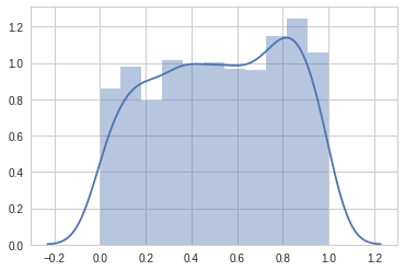

png

# Let's plot normal distribution

x = random.randn(100000)
sns.set_style('whitegrid')
sns.distplot(x)

/usr/local/lib/python3.6/dist-packages/matplotlib/axes/_axes.py:6521: MatplotlibDeprecationWarning: 
The 'normed' kwarg was deprecated in Matplotlib 2.1 and will be removed in 3.1. Use 'density' instead.
  alternative="'density'", removal="3.1")





<matplotlib.axes._subplots.AxesSubplot at 0x7f03f68a1518>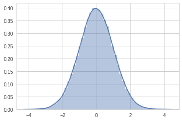

png

# Let's plot poisson distribution

x = random.poisson(5, 1000)
sns.set_style('whitegrid')
sns.distplot(x)

/usr/local/lib/python3.6/dist-packages/matplotlib/axes/_axes.py:6521: MatplotlibDeprecationWarning: 
The 'normed' kwarg was deprecated in Matplotlib 2.1 and will be removed in 3.1. Use 'density' instead.
  alternative="'density'", removal="3.1")





<matplotlib.axes._subplots.AxesSubplot at 0x7f03f4739470>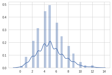

png

diag

# a diagonal matrix
diag([1,2,3])

array([[1, 0, 0],
       [0, 2, 0],
       [0, 0, 3]])

# diagonal with offset from the main diagonal
diag([1,2,3], k=1)

array([[0, 1, 0, 0],
       [0, 0, 2, 0],
       [0, 0, 0, 3],
       [0, 0, 0, 0]])

zeroes and ones

zeros((3,3))

array([[0., 0., 0.],
       [0., 0., 0.],
       [0., 0., 0.]])

ones((3,3))

array([[1., 1., 1.],
       [1., 1., 1.],
       [1., 1., 1.]])

File IO

Comma-separated values (CSV)

A very common file format for data files is comma-separated values (CSV), or related formats such as TSV (tab-separated values). To read data from such files into Numpy arrays we can use the numpy.genfromtxt function. For example:

!wget https://raw.githubusercontent.com/jrjohansson/scientific-python-lectures/master/stockholm_td_adj.dat

--2019-01-23 18:17:43--  https://raw.githubusercontent.com/jrjohansson/scientific-python-lectures/master/stockholm_td_adj.dat
Resolving raw.githubusercontent.com (raw.githubusercontent.com)... 151.101.0.133, 151.101.64.133, 151.101.128.133, ...
Connecting to raw.githubusercontent.com (raw.githubusercontent.com)|151.101.0.133|:443... connected.
HTTP request sent, awaiting response... 200 OK
Length: 2864946 (2.7M) [text/plain]
Saving to: ‘stockholm_td_adj.dat’

stockholm_td_adj.da 100%[===================>]   2.73M  --.-KB/s    in 0.06s   

2019-01-23 18:17:43 (43.9 MB/s) - ‘stockholm_td_adj.dat’ saved [2864946/2864946]

!head stockholm_td_adj.dat

1800  1  1    -6.1    -6.1    -6.1 1
1800  1  2   -15.4   -15.4   -15.4 1
1800  1  3   -15.0   -15.0   -15.0 1
1800  1  4   -19.3   -19.3   -19.3 1
1800  1  5   -16.8   -16.8   -16.8 1
1800  1  6   -11.4   -11.4   -11.4 1
1800  1  7    -7.6    -7.6    -7.6 1
1800  1  8    -7.1    -7.1    -7.1 1
1800  1  9   -10.1   -10.1   -10.1 1
1800  1 10    -9.5    -9.5    -9.5 1

data = genfromtxt('stockholm_td_adj.dat')

data.shape

(77431, 7)

fig, ax = plt.subplots(figsize=(14,4))
ax.plot(data[:,0]+data[:,1]/12.0+data[:,2]/365, data[:,5])
ax.axis('tight')
ax.set_title('tempeatures in Stockholm')
ax.set_xlabel('year')
ax.set_ylabel('temperature (C)');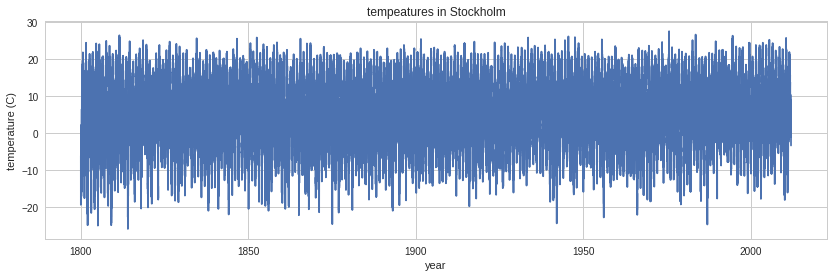

png

Using numpy.savetxt we can store a Numpy array to a file in CSV format:

M = random.rand(3,3)

M

array([[0.15899226, 0.73913852, 0.0858632 ],
       [0.41821712, 0.11712784, 0.34176831],
       [0.52685163, 0.12873943, 0.92178189]])

savetxt("random-matrix.csv", M)

!cat random-matrix.csv

1.589922582398127782e-01 7.391385219751671620e-01 8.586320111848333436e-02
4.182171214227743405e-01 1.171278378058918657e-01 3.417683058329642476e-01
5.268516328643041424e-01 1.287394330466531400e-01 9.217818880426476014e-01

savetxt("random-matrix.csv", M, fmt='%.5f') # fmt specifies the format

!cat random-matrix.csv

0.15899 0.73914 0.08586
0.41822 0.11713 0.34177
0.52685 0.12874 0.92178

Numpy’s native file format

Useful when storing and reading back numpy array data. Use the functions numpy.save and numpy.load:

save("random-matrix.npy", M)

!ls -lh *

-rw-r--r-- 1 root root   72 Jan 23 18:19 random-matrix.csv
-rw-r--r-- 1 root root  200 Jan 23 18:19 random-matrix.npy
-rw-r--r-- 1 root root 2.8M Jan 23 18:17 stockholm_td_adj.dat

sample_data:
total 55M
-r-xr-xr-x 1 root root 1.7K Jan  1  2000 anscombe.json
-rw-r--r-- 1 root root 295K Jan  8 17:14 california_housing_test.csv
-rw-r--r-- 1 root root 1.7M Jan  8 17:14 california_housing_train.csv
-rw-r--r-- 1 root root  18M Jan  8 17:15 mnist_test.csv
-rw-r--r-- 1 root root  35M Jan  8 17:15 mnist_train_small.csv
-r-xr-xr-x 1 root root  903 Jan  1  2000 README.md

Manipulating arrays

Indexing

We can index elements in an array using square brackets and indices:

# vector, and has only one dimension, taking one index
vector[0]

# matrix is a 2 dimensional array, taking two indices 
matrix[1,1]

4.0

If we omit an index of a multidimensional array it returns the whole row (or, in general, a N-1 dimensional array)

matrix

array([[1., 2.],
       [3., 4.]])

matrix[1]

array([3., 4.])

The same thing can be achieved with using : instead of an index:

matrix[1,:] #row 1

array([3., 4.])

matrix[:,1] #column 1

array([2., 4.])

We can assign new values to elements in an array using indexing:

matrix[1,1] = 1

matrix

array([[1., 2.],
       [3., 1.]])

# also works for rows and columns
matrix[1,:] = 0
matrix[:,1] = -1

matrix

array([[ 1., -1.],
       [ 0., -1.]])

Index slicing

Index slicing is the technical name for the syntax M[lower:upper:step] to extract part of an array:

A = array([1,2,3,4,5])
A

array([1, 2, 3, 4, 5])

A[1:3] = [-2,-3]

A

array([ 1, -2, -3,  4,  5])

A[::] # lower, upper, step all take the default values

array([ 1, -2, -3,  4,  5])

A[::2] # step is 2, lower and upper defaults to the beginning and end of the array

array([ 1, -3,  5])

A[:3] # first three elements

array([ 1, -2, -3])

A[3:] # elements from index 3

array([4, 5])

Negative indices counts from the end of the array (positive index from the begining):

A = array([1,2,3,4,5])

A[-1] # the last element in the array

A[-3:] # the last three elements

array([3, 4, 5])

Index slicing works exactly the same way for multidimensional arrays:

A = array([[n+m*10 for n in range(5)] for m in range(5)])

A

array([[ 0,  1,  2,  3,  4],
       [10, 11, 12, 13, 14],
       [20, 21, 22, 23, 24],
       [30, 31, 32, 33, 34],
       [40, 41, 42, 43, 44]])

# a block from the original array
A[1:4, 1:4]

array([[11, 12, 13],
       [21, 22, 23],
       [31, 32, 33]])

# strides
A[::2, ::2]

array([[ 0,  2,  4],
       [20, 22, 24],
       [40, 42, 44]])

Fancy indexing

Fancy indexing is the name for when an array or list is used in-place of an index:

row_indices = [1, 2, 3]
A[row_indices]

array([[10, 11, 12, 13, 14],
       [20, 21, 22, 23, 24],
       [30, 31, 32, 33, 34]])

col_indices = [1, 2, -1] # remember, index -1 means the last element
A[row_indices, col_indices]

array([11, 22, 34])

We can also use index masks: If the index mask is an Numpy array of data type bool, then an element is selected (True) or not (False) depending on the value of the index mask at the position of each element:

B = array([n for n in range(5)])
B

array([0, 1, 2, 3, 4])

row_mask = array([True, False, True, False, False])
B[row_mask]

array([0, 2])

# same thing
row_mask = array([1,0,1,0,0], dtype=bool)
B[row_mask]

array([0, 2])

This feature is very useful to conditionally select elements from an array, using for example comparison operators:

x = arange(0, 10, 0.5)
x

array([0. , 0.5, 1. , 1.5, 2. , 2.5, 3. , 3.5, 4. , 4.5, 5. , 5.5, 6. ,
       6.5, 7. , 7.5, 8. , 8.5, 9. , 9.5])

mask = (5 < x) * (x < 7.5)
mask

array([False, False, False, False, False, False, False, False, False,
       False, False,  True,  True,  True,  True, False, False, False,
       False, False])

x[mask]

array([5.5, 6. , 6.5, 7. ])

( 5 < x ) * (x < 7.5)

array([False, False, False, False, False, False, False, False, False,
       False, False,  True,  True,  True,  True, False, False, False,
       False, False])

Functions for extracting data from arrays and creating arrays

where

The index mask can be converted to position index using the where function

indices = where(mask)

indices

(array([11, 12, 13, 14]),)

x[indices] # this indexing is equivalent to the fancy indexing x[mask]

array([5.5, 6. , 6.5, 7. ])

####diag With the diag function we can also extract the diagonal and subdiagonals of an array:

array([[ 0,  1,  2,  3,  4],
       [10, 11, 12, 13, 14],
       [20, 21, 22, 23, 24],
       [30, 31, 32, 33, 34],
       [40, 41, 42, 43, 44]])

diag(A)

array([ 0, 11, 22, 33, 44])

diag(A, -1)

array([10, 21, 32, 43])

take

The take function is similar to fancy indexing described above:

v2 = arange(-3,3)
v2

array([-3, -2, -1,  0,  1,  2])

row_indices = [1, 3, 5]
v2[row_indices] # fancy indexing

array([-2,  0,  2])

v2.take(row_indices)

array([-2,  0,  2])

But take also works on lists and other objects:

take([-3, -2, -1,  0,  1,  2], row_indices)

array([-2,  0,  2])

####choose Constructs an array by picking elements from several arrays:

which = [1, 0, 1, 0]
choices = [[1,2,3,4], [-1,-2,-3,-4]]

choose(which, choices)

array([-1,  2, -3,  4])

Linear algebra

Vectorizing code is the key to writing efficient numerical calculation with Python/Numpy. That means that as much as possible of a program should be formulated in terms of matrix and vector operations, like matrix-matrix multiplication.

Scalar-array operations

We can use the usual arithmetic operators to multiply, add, subtract, and divide arrays with scalar numbers.

v1 = arange(0, 5)

v1

array([0, 1, 2, 3, 4])

v1 * 2

array([0, 2, 4, 6, 8])

v1 + 2

array([2, 3, 4, 5, 6])

array([[ 0,  1,  2,  3,  4],
       [10, 11, 12, 13, 14],
       [20, 21, 22, 23, 24],
       [30, 31, 32, 33, 34],
       [40, 41, 42, 43, 44]])

A * 2

array([[ 0,  2,  4,  6,  8],
       [20, 22, 24, 26, 28],
       [40, 42, 44, 46, 48],
       [60, 62, 64, 66, 68],
       [80, 82, 84, 86, 88]])

A + 2

array([[ 2,  3,  4,  5,  6],
       [12, 13, 14, 15, 16],
       [22, 23, 24, 25, 26],
       [32, 33, 34, 35, 36],
       [42, 43, 44, 45, 46]])

Element-wise array-array operations

When we add, subtract, multiply and divide arrays with each other, the default behaviour is element-wise operations:

v1 * v1

array([ 0,  1,  4,  9, 16])

A * A

array([[   0,    1,    4,    9,   16],
       [ 100,  121,  144,  169,  196],
       [ 400,  441,  484,  529,  576],
       [ 900,  961, 1024, 1089, 1156],
       [1600, 1681, 1764, 1849, 1936]])

If we multiply arrays with compatible shapes, we get an element-wise multiplication of each row:

A.shape

(5, 5)

v1.shape

(5,)

v1

array([0, 1, 2, 3, 4])

array([[ 0,  1,  2,  3,  4],
       [10, 11, 12, 13, 14],
       [20, 21, 22, 23, 24],
       [30, 31, 32, 33, 34],
       [40, 41, 42, 43, 44]])

A * v1

array([[  0,   1,   4,   9,  16],
       [  0,  11,  24,  39,  56],
       [  0,  21,  44,  69,  96],
       [  0,  31,  64,  99, 136],
       [  0,  41,  84, 129, 176]])

v1 * A

array([[  0,   1,   4,   9,  16],
       [  0,  11,  24,  39,  56],
       [  0,  21,  44,  69,  96],
       [  0,  31,  64,  99, 136],
       [  0,  41,  84, 129, 176]])

Matrix algebra

What about matrix mutiplication? There are two ways. We can either use the dot function, which applies a matrix-matrix, matrix-vector, or inner vector multiplication to its two arguments:

Dot multiplication:

$a\cdot b=\sum_{i=1}^n a_n b_n = a_1 b_1 + a_2 b_2 + … + a_n b_n$

array([[ 0,  1,  2,  3,  4],
       [10, 11, 12, 13, 14],
       [20, 21, 22, 23, 24],
       [30, 31, 32, 33, 34],
       [40, 41, 42, 43, 44]])

dot(A,A)

array([[ 300,  310,  320,  330,  340],
       [1300, 1360, 1420, 1480, 1540],
       [2300, 2410, 2520, 2630, 2740],
       [3300, 3460, 3620, 3780, 3940],
       [4300, 4510, 4720, 4930, 5140]])

t = array([[1,2],[3,4]])

array([[1, 2],
       [3, 4]])

dot(t,t)

array([[ 7, 10],
       [15, 22]])

z = array([1,2,3])
dot(z,z)

dot([1,2],[1,3])

v1

array([0, 1, 2, 3, 4])

dot(A,v1)

array([ 30, 130, 230, 330, 430])

from numpy.linalg import *

array([[ 0,  1,  2,  3,  4],
       [10, 11, 12, 13, 14],
       [20, 21, 22, 23, 24],
       [30, 31, 32, 33, 34],
       [40, 41, 42, 43, 44]])

a = array([[[1., 2.], [3., 4.]], [[1, 3], [3, 5]]])

Data processing

Often it is useful to store datasets in Numpy arrays. Numpy provides a number of functions to calculate statistics of datasets in arrays.

For example, let’s calculate some properties from the Stockholm temperature dataset used above.

# reminder, the tempeature dataset is stored in the data variable:
shape(data)

(77431, 7)

####mean

# the temperature data is in column 3
mean(data[:,3])

6.197109684751585

The daily mean temperature in Stockholm over the last 200 years has been about 6.2 C.

SD and variance

std(data[:,3]), var(data[:,3])

(8.282271621340573, 68.59602320966341)

####min and max

# lowest daily average temperature
data[:,3].min()

-25.8

# highest daily average temperature
data[:,3].max()

28.3

sum, prod, and trace

d = arange(0, 10)
d

array([0, 1, 2, 3, 4, 5, 6, 7, 8, 9])

# sum up all elements
sum(d)

# product of all elements
prod(d+1)

d+1

array([ 1,  2,  3,  4,  5,  6,  7,  8,  9, 10])

# cummulative product
cumprod(d+1)

array([      1,       2,       6,      24,     120,     720,    5040,
         40320,  362880, 3628800])

# same as: diag(A).sum()
trace(A)

Calculations with higher-dimensional data

When functions such as min, max, etc. are applied to a multidimensional arrays, it is sometimes useful to apply the calculation to the entire array, and sometimes only on a row or column basis. Using the axis argument we can specify how these functions should behave:

m = random.rand(3,3)
m

array([[0.33829171, 0.40448773, 0.53537406],
       [0.70139575, 0.82815424, 0.75878347],
       [0.52038369, 0.03975169, 0.67270888]])

# global max
m.max()

0.8281542387464986

# max in each column
m.max(axis=0)

array([0.70139575, 0.82815424, 0.75878347])

# max in each row
m.max(axis=1)

array([0.53537406, 0.82815424, 0.67270888])

Many other functions and methods in the array and matrix classes accept the same (optional) axis keyword argument.

Reshaping, resizing and stacking arrays

The shape of an Numpy array can be modified without copying the underlaying data, which makes it a fast operation even for large arrays.

array([[ 0,  1,  2,  3,  4],
       [10, 11, 12, 13, 14],
       [20, 21, 22, 23, 24],
       [30, 31, 32, 33, 34],
       [40, 41, 42, 43, 44]])

A.shape

(5, 5)

n, m = A.shape

B = A.reshape((1,n*m))

array([[ 0,  1,  2,  3,  4, 10, 11, 12, 13, 14, 20, 21, 22, 23, 24, 30,
        31, 32, 33, 34, 40, 41, 42, 43, 44]])

B[0,0:5] = 5

array([[ 5,  5,  5,  5,  5, 10, 11, 12, 13, 14, 20, 21, 22, 23, 24, 30,
        31, 32, 33, 34, 40, 41, 42, 43, 44]])

array([[ 5,  5,  5,  5,  5],
       [10, 11, 12, 13, 14],
       [20, 21, 22, 23, 24],
       [30, 31, 32, 33, 34],
       [40, 41, 42, 43, 44]])

We can also use the function flatten to make a higher-dimensional array into a vector. But this function create a copy of the data.

B = A.flatten()

B

array([ 5,  5,  5,  5,  5, 10, 11, 12, 13, 14, 20, 21, 22, 23, 24, 30, 31,
       32, 33, 34, 40, 41, 42, 43, 44])

B[0:5] = 10

B

array([10, 10, 10, 10, 10, 10, 11, 12, 13, 14, 20, 21, 22, 23, 24, 30, 31,
       32, 33, 34, 40, 41, 42, 43, 44])

array([[ 5,  5,  5,  5,  5],
       [10, 11, 12, 13, 14],
       [20, 21, 22, 23, 24],
       [30, 31, 32, 33, 34],
       [40, 41, 42, 43, 44]])

Adding a new dimension: newaxis

With newaxis, we can insert new dimensions in an array, for example converting a vector to a column or row matrix:

v = array([1,2,3])

shape(v)

(3,)

# make a column matrix of the vector v
v[:, newaxis]

array([[1],
       [2],
       [3]])

v[newaxis,:]

array([[1, 2, 3]])

v[newaxis,:].shape

(1, 3)

Stacking and repeating arrays

Using function repeat,tile, vstack, hstack, and concatenate we can create larger vectors and matrices from smaller ones:

####tile and repeat

a = array([[1, 2], [3, 4]])

# repeat each element 3 times
repeat(a, 3)

array([1, 1, 1, 2, 2, 2, 3, 3, 3, 4, 4, 4])

# tile the matrix 3 times 
tile(a, 3)

array([[1, 2, 1, 2, 1, 2],
       [3, 4, 3, 4, 3, 4]])

####concatenate

b = array([[5, 6]])

concatenate((a, b), axis=0)

array([[1, 2],
       [3, 4],
       [5, 6]])

b.T

array([[5],
       [6]])

concatenate((a, b.T), axis=1)

array([[1, 2, 5],
       [3, 4, 6]])

####vertical and horizontal stack

vstack((a,b))

array([[1, 2],
       [3, 4],
       [5, 6]])

hstack((a,b.T))

array([[1, 2, 5],
       [3, 4, 6]])

Copy versus “deep copy”

To achieve high performance, assignments in Python usually do not copy the underlaying objects. This is important for example when objects are passed between functions, to avoid an excessive amount of memory copying when it is not necessary (technical term: pass by reference).

A = array([[1, 2], [3, 4]])

A

array([[1, 2],
       [3, 4]])

# now B is referring to the same array data as A 
B = A

# changing B affects A
B[0,0] = 10

B

array([[10,  2],
       [ 3,  4]])

array([[10,  2],
       [ 3,  4]])

If we want to avoid this behavior, so that when we get a new completely independent object B copied from A, then we need to do a so-called “deep copy” using the function copy:

B = copy(A)

# now, if we modify B, A is not affected
B[0,0] = -5

B

array([[-5,  2],
       [ 3,  4]])

array([[10,  2],
       [ 3,  4]])

Iterating over array elements

Generally, we want to avoid iterating over the elements of arrays whenever we can (at all costs). The reason is that in a interpreted language like Python (or MATLAB), iterations are really slow compared to vectorized operations.

However, sometimes iterations are unavoidable. For such cases, the Python for loop is the most convenient way to iterate over an array:

v = array([1,2,3,4])

for element in v:
    print(element)

M = array([[1,2], [3,4]])

for row in M:
    print("row", row)
    
    for element in row:
        print(element)

row [1 2]
1
2
row [3 4]
3
4

When we need to iterate over each element of an array and modify its elements, it is convenient to use the enumerate function to obtain both the element and its index in the for loop:

for row_idx, row in enumerate(M):
    print("row_idx", row_idx, "row", row)
    
    for col_idx, element in enumerate(row):
        print("col_idx", col_idx, "element", element)
       
        # update the matrix M: square each element
        M[row_idx, col_idx] = element ** 2

row_idx 0 row [1 2]
col_idx 0 element 1
col_idx 1 element 2
row_idx 1 row [3 4]
col_idx 0 element 3
col_idx 1 element 4

# each element in M is now squared
M

array([[ 1,  4],
       [ 9, 16]])

Using arrays in conditions

When using arrays in conditions,for example if statements and other boolean expressions, one needs to use any or all, which requires that any or all elements in the array evalutes to True:

array([[ 1,  4],
       [ 9, 16]])

if (M > 5).any():
    print("at least one element in M is larger than 5")
else:
    print("no element in M is larger than 5")

at least one element in M is larger than 5

if (M > 5).all():
    print("all elements in M are larger than 5")
else:
    print("all elements in M are not larger than 5")

all elements in M are not larger than 5

M[any(M>5,axis=1)]

array([[ 9, 16]])

Type casting

Since Numpy arrays are statically typed, the type of an array does not change once created. But we can explicitly cast an array of some type to another using the astype functions (see also the similar asarray function). This always create a new array of new type:

M.dtype

dtype('int64')

M2 = M.astype(float)

M2

array([[ 1.,  4.],
       [ 9., 16.]])

M2.dtype

dtype('float64')

M3 = M.astype(bool)

M3

array([[ True,  True],
       [ True,  True]])

Homework 1 with numpy

# Get the datasets
!wget https://nekrut.github.io/BMMB554/yeast_genes.txt

--2019-01-23 18:23:32--  https://nekrut.github.io/BMMB554/yeast_genes.txt
Resolving nekrut.github.io (nekrut.github.io)... 185.199.109.153, 185.199.110.153, 185.199.111.153, ...
Connecting to nekrut.github.io (nekrut.github.io)|185.199.109.153|:443... connected.
HTTP request sent, awaiting response... 200 OK
Length: 236742 (231K) [text/plain]
Saving to: ‘yeast_genes.txt’

yeast_genes.txt     100%[===================>] 231.19K  --.-KB/s    in 0.03s   

2019-01-23 18:23:32 (7.88 MB/s) - ‘yeast_genes.txt’ saved [236742/236742]

!cut -f 3 yeast_genes.txt | sort | uniq -c

    131 chrI
    485 chrII
    253 chrIII
    889 chrIV
    264 chrIX
     58 chrmt
      1 chrom
    360 chrV
    161 chrVI
    642 chrVII
    340 chrVIII
    438 chrX
    375 chrXI
    644 chrXII
    551 chrXIII
    459 chrXIV
    640 chrXV
    548 chrXVI

# First let's find out how many chromosomes:
chrom = []
for line in open('yeast_genes.txt','r'):
  if not line.startswith('#'): # ignore header
    chrom.append(line.split('\t')[2]) #split line on tabs and access the third [2] element
set(chrom)

{'chrI',
 'chrII',
 'chrIII',
 'chrIV',
 'chrIX',
 'chrV',
 'chrVI',
 'chrVII',
 'chrVIII',
 'chrX',
 'chrXI',
 'chrXII',
 'chrXIII',
 'chrXIV',
 'chrXV',
 'chrXVI',
 'chrmt'}

# Let's create two arrays to translate between roman and integer
# The trick here is than index of every element can be used to
# Translate roman into integer
# For example, chr_roman[1] is 'chrI'

chr_roman = ['chrmt',
 'chrI',       
 'chrII',
 'chrIII',
 'chrIV',
 'chrV',
 'chrVI',
 'chrVII',
 'chrVIII',
 'chrIX',
 'chrX',
 'chrXI',
 'chrXII',
 'chrXIII',
 'chrXIV',
 'chrXV',
 'chrXVI']

chr_roman.index('chrI')

# Process the dataset

names = [] # Initialize array for gene names
coord = [] # Initialize array for coordinate data

for line in open('yeast_genes.txt','r'):
  if not line.startswith('#'): # ignore header
    line = line.rstrip() # get rid of caret returns
    fields = line.split('\t') # split line on tabs to convert it into a list
    name = fields[0]
    chromosome = chr_roman.index(fields[2])
    start = int( fields[3] )
    end = int( fields[4] )
    length = end-start+1 # compute the length
    if name.split('-')[0].endswith('W'):
      strand = 1 # encode positive strand as 1
    elif name.split('-')[0].endswith('C'):
      strand = 2 # encode negative strand as 2
    else:        
      strand = 0 # encode unknown strand as 0
    names.append(name)
    coord.append([chromosome,start,end,length,strand])

coord[:2]

[[0, 61868, 62447, 580, 0], [0, 1, 11, 11, 0]]

names[:2]

['21S_rRNA_4', '9S_rRNA_1']

!head -n 3 yeast_genes.txt

#systematic_name    standard_name   chrom   start   end
21S_rRNA_4  21S_RRNA_4  chrmt   61868   62447
9S_rRNA_1   9S_RRNA_1   chrmt   1   11

# Convert coord array into numpy array
coord = array(coord)

coord[:2]

array([[    0, 61868, 62447,   580,     0],
       [    0,     1,    11,    11,     0]])

coord.dtype

dtype('int64')

# Convert names array into numpy array
names = array(names)

names[:2]

array(['21S_rRNA_4', '9S_rRNA_1'], dtype='<U10')

# The number of genes can be inferred from array shape
coord.shape

(7238, 5)

# You can see that the file as many lines + 1 (header)
!wc -l yeast_genes.txt

7239 yeast_genes.txt

# Longest gene is the max of the dufference between start and end
max(coord[:,2] - coord[:,1] + 1)

# Or simply the maximum of the length column
max(coord[:,3])

# Which gene is that?
# The index of this gene in coord array is:
argmax(coord[:,3])

# It has the same index in names array:
names[4740]

'YLR106C'

# Shortest gene
min(coord[:,3])

# The number of genes on chromsome 10
shape(extract(coord[:,0] == 10,coord))

(438,)

# Longest gene on chromosome 10
max(extract(coord[:,0] == 10,coord[:,3]))

# The number of genes of chromsome 1 that are on the + strand 
# (we encoded '+' as 1)
size(coord[(coord[:,0] == 1) & (coord[:,4] == 1)], axis=0)

# The number of genes of chromsome 1 that are on the - strand 
# (we encoded '-' as 2)
size(coord[(coord[:,0] == 1) & (coord[:,4] == 2)], axis=0)

# Let's plot distribution of gene lengths
sns.set_style('whitegrid')
sns.distplot(coord[:,3])

/usr/local/lib/python3.6/dist-packages/matplotlib/axes/_axes.py:6521: MatplotlibDeprecationWarning: 
The 'normed' kwarg was deprecated in Matplotlib 2.1 and will be removed in 3.1. Use 'density' instead.
  alternative="'density'", removal="3.1")





<matplotlib.axes._subplots.AxesSubplot at 0x7f03f238c6a0>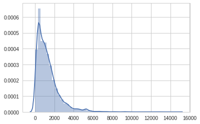

png

A little fun with images

Images are really arrays

import matplotlib.pyplot as pl
import matplotlib.image as mpimg
import numpy as np

import imageio
img="https://nekrut.github.io/BMMB554/img/1N1A6336.CR2.jpg"
img = imageio.imread(img)

img.shape

(880, 1320, 3)

start_img[0]

---------------------------------------------------------------------------

NameError                                 Traceback (most recent call last)

<ipython-input-200-ccafdea59cf4> in <module>()
----> 1 start_img[0]


NameError: name 'start_img' is not defined

plt.imshow(img,cmap=plt.cm.gray)
plt.axis('off')

(-0.5, 1319.5, 879.5, -0.5)

png

flip = np.flipud(img)

plt.imshow(flip)
plt.axis('off')

(-0.5, 1319.5, 879.5, -0.5)

png